library(analogsea)
library(plumber)
library(plumberDeploy)
library(remotes)
library(ssh)
library(tidymodels)
library(tidyverse)Online Appendix I — Production
Prerequisites
- Read Science Storms the Cloud, (Gentemann et al. 2021)
- Describes the importance of being able to compute using the cloud.
- Read Machine learning is going real-time, (Huyen 2020)
- Discussion of the need to be able to make forecasts on the fly.
- Watch Democratizing R with Plumber APIs, (Blair 2019)
- Overview of using
plumberto make an API.
- Overview of using
- Read Operationalizing Machine Learning: An Interview Study, (Shankar et al. 2022).
- Provides the results of interviews with machine learning engineers.
Key concepts and skills
- Putting a model into production - i.e. using it in a real-world setting - requires an additional set of skills, including a familiarity with a cloud provider and the ability to create an API.
Software and packages
analogsea(Chamberlain et al. 2022)plumber(Schloerke and Allen 2022)plumberDeploy(Allen 2021)remotes(Csárdi et al. 2021)ssh(Ooms 2022)tidymodels(Kuhn and Wickham 2020)tidyverse(Wickham et al. 2019)
I.1 Introduction
Having done the work to develop a dataset and explore it with a model that we are confident can be used, we may wish to enable this to be used more widely than just our own computer. There are a variety of ways of doing this, including:
- using the cloud;
- creating R packages;
- making
shinyapplications; and - using
plumberto create an API.
The general idea here is that we need to know, and allow others to come to trust, the whole workflow. That is what our approach to this point brings. After this, then we may like to use our model more broadly. Say we have been able to scrape some data from a website, bring some order to that chaos, make some charts, appropriately model it, and write this all up. In most academic settings that is more than enough. But in many industry settings we would like to use the model to do something. For instance, setting up a website that allows a model to be used to generate an insurance quote given several inputs.
In this chapter, we begin by moving our compute from our local computer to the cloud. We then describe the use of R packages and Shiny for sharing models. That works well, but in some settings other users may like to interact with our model in ways that we are not focused on. One way to allow this is to make our results available to other computers, and for that we will want to make an API. Hence, we introduce plumber (Schloerke and Allen 2022), which is a way of creating APIs.
I.2 Amazon Web Services
Apocryphally the cloud is just another name for someone else’s computer. And while that is true to various degrees, for our purposes that is enough. Learning to use someone else’s computer can be great for a number of reasons including:
- Scalability: It can be quite expensive to buy a new computer, especially if we only need it to run something every now and then, but by using the cloud, we can just rent for a few hours or days. This allows use to amortize this cost and work out what we actually need before committing to a purchase. It also allows us to easily increase or decrease the compute scale if we suddenly have a substantial increase in demand.
- Portability: If we can shift our analysis workflow from a local computer to the cloud, then that suggests that we are likely doing good things in terms of reproducibility and portability. At the very least, code can run both locally and on the cloud, which is a big step in terms of reproducibility.
- Set-and-forget: If we are doing something that will take a while, then it can be great to not have to worry about our own computer needing to run overnight. Additionally, on many cloud options, open-source statistical software, such as R and Python, is either already available, or relatively easy to set up.
That said, there are downsides, including:
- Cost: While most cloud options are cheap, they are rarely free. To provide an idea of cost, using a well-featured AWS instance for a few days may end up being a few dollars. It is also easy to accidentally forget about something, and generate unexpectedly large bills, especially initially.
- Public: It can be easy to make mistakes and accidentally make everything public.
- Time: It takes time to get set up and comfortable on the cloud.
When we use the cloud, we are typically running code on a “virtual machine” (VM). This is an allocation that is part of a larger collection of computers that has been designed to act like a computer with specific features. For instance, we may specify that our virtual machine has, say, 8GB RAM, 128GB storage, and 4 CPUs. The VM would then act like a computer with those specifications. The cost to use cloud options increases based on the VM specifications.
In a sense, we started with a cloud option, through our initial recommendation in Chapter 2 of using Posit Cloud, before we moved to our local computer in Appendix A. That cloud option was specifically designed for beginners. We will now introduce a more general cloud option: Amazon Web Services (AWS). Often a particular business will use a particular cloud option, such as Google, AWS, or Azure, but developing familiarity with one will make the use of the others easier.
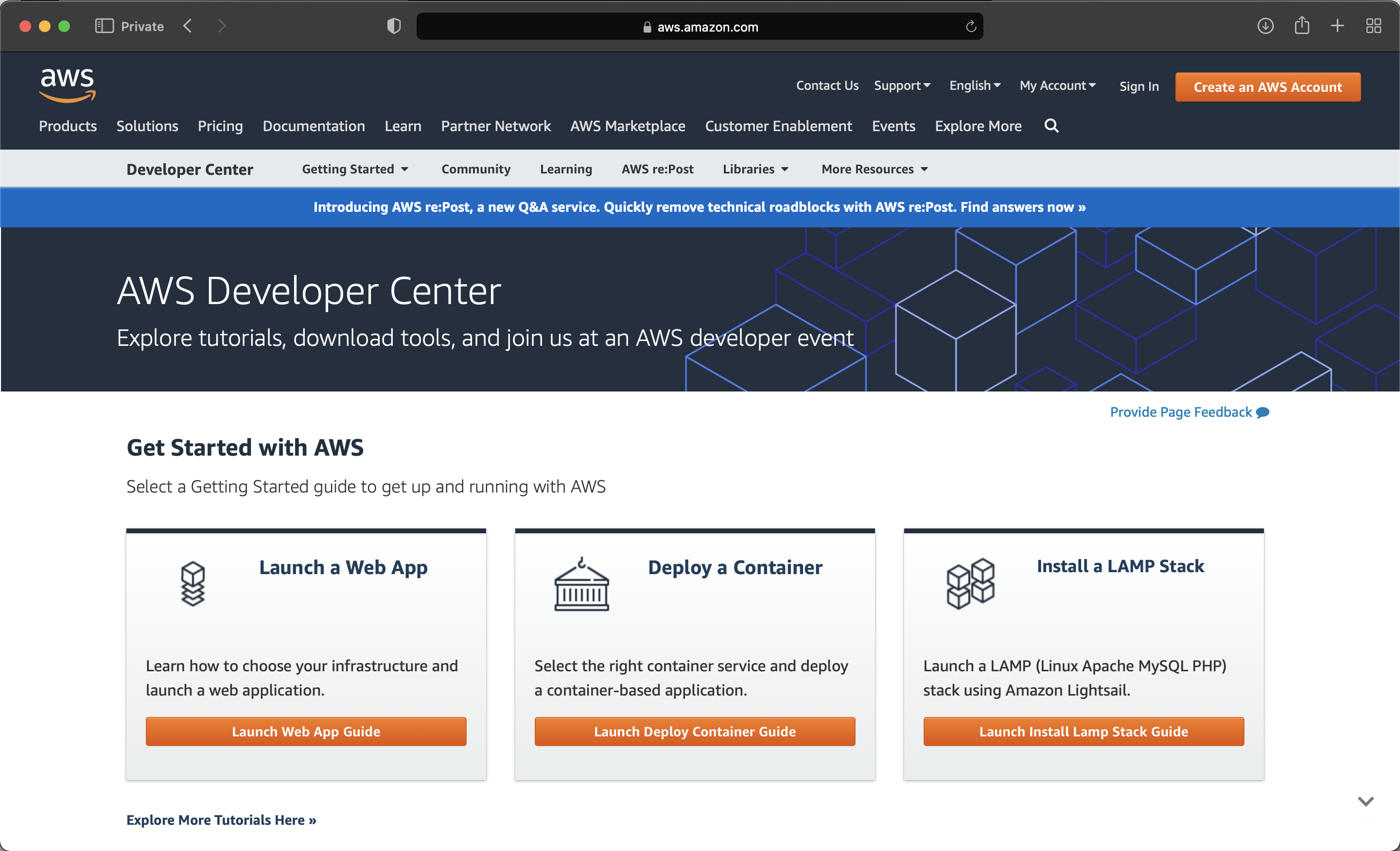
Amazon Web Services is a cloud service from Amazon. To get started we need to create an AWS Developer account here (Figure I.1 (a)).
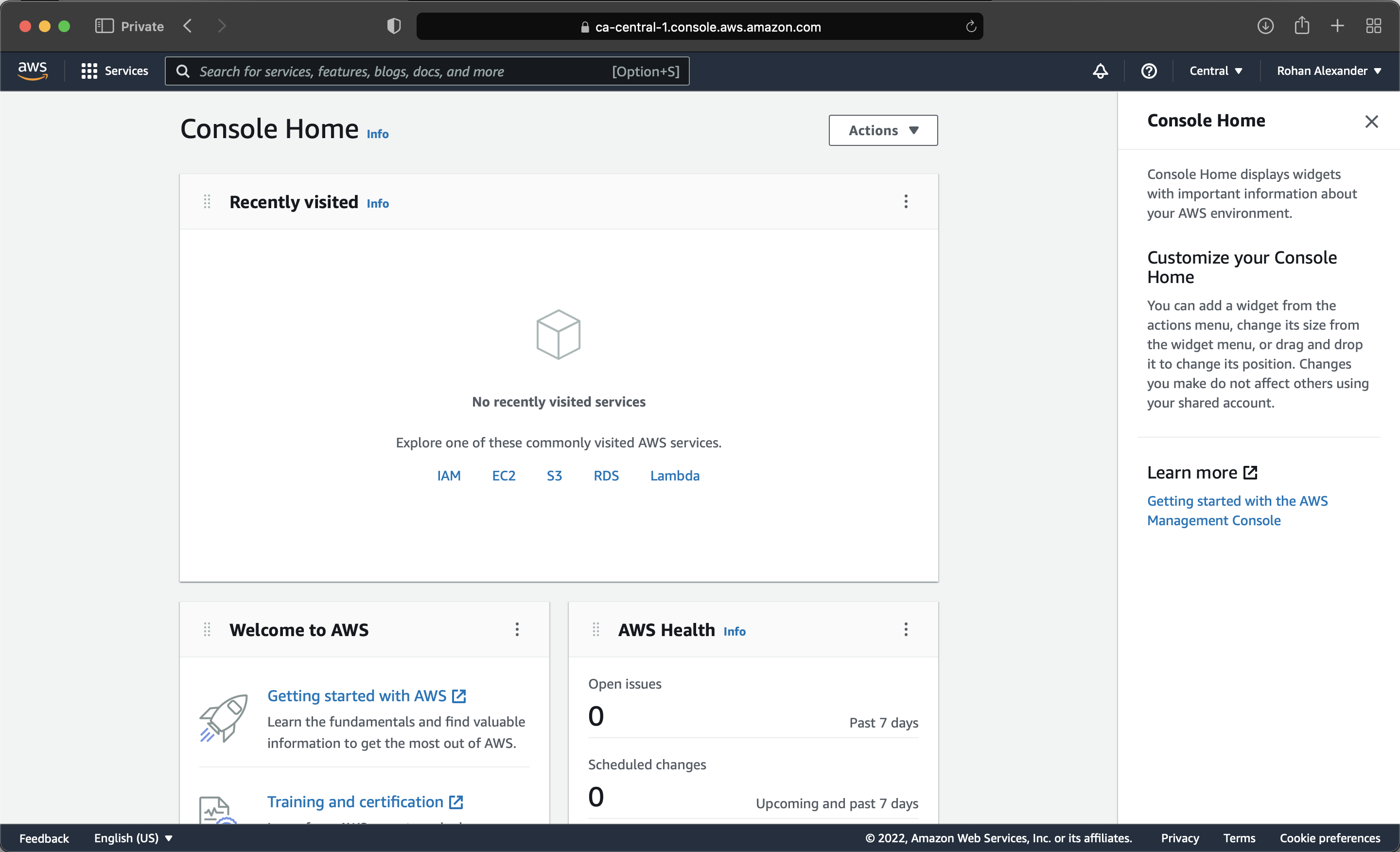
After we have created an account, we need to select a region where the computer that we will access is located. After this, we want to “Launch a virtual machine” with EC2 (Figure I.1 (b)).
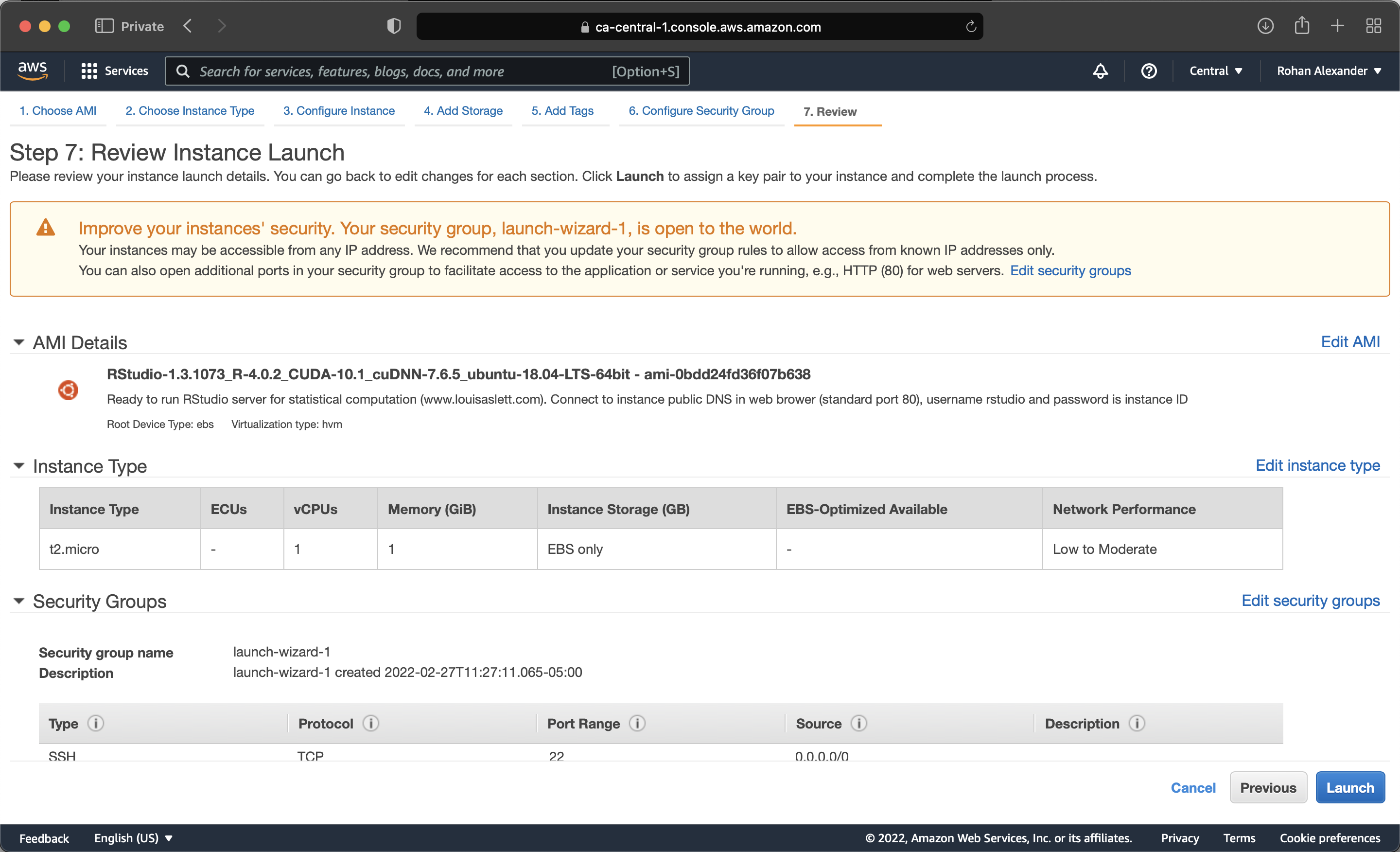
The first step is to choose an Amazon Machine Image (AMI). This provides the details of the computer that you will be using. For instance, a local computer may be a MacBook running Monterey. Louis Aslett provides AMIs that are already set up with RStudio and much else here. We can either search for the AMI of the region that we registered for, or click on the relevant link on Aslett’s website. For instance, to use the AMI set-up for the Canadian central region we search for “ami-0bdd24fd36f07b638”. The benefit of using these AMIs is that they are set up specifically for RStudio, but the trade-off is that they are a little outdated, as they were compiled in August 2020.
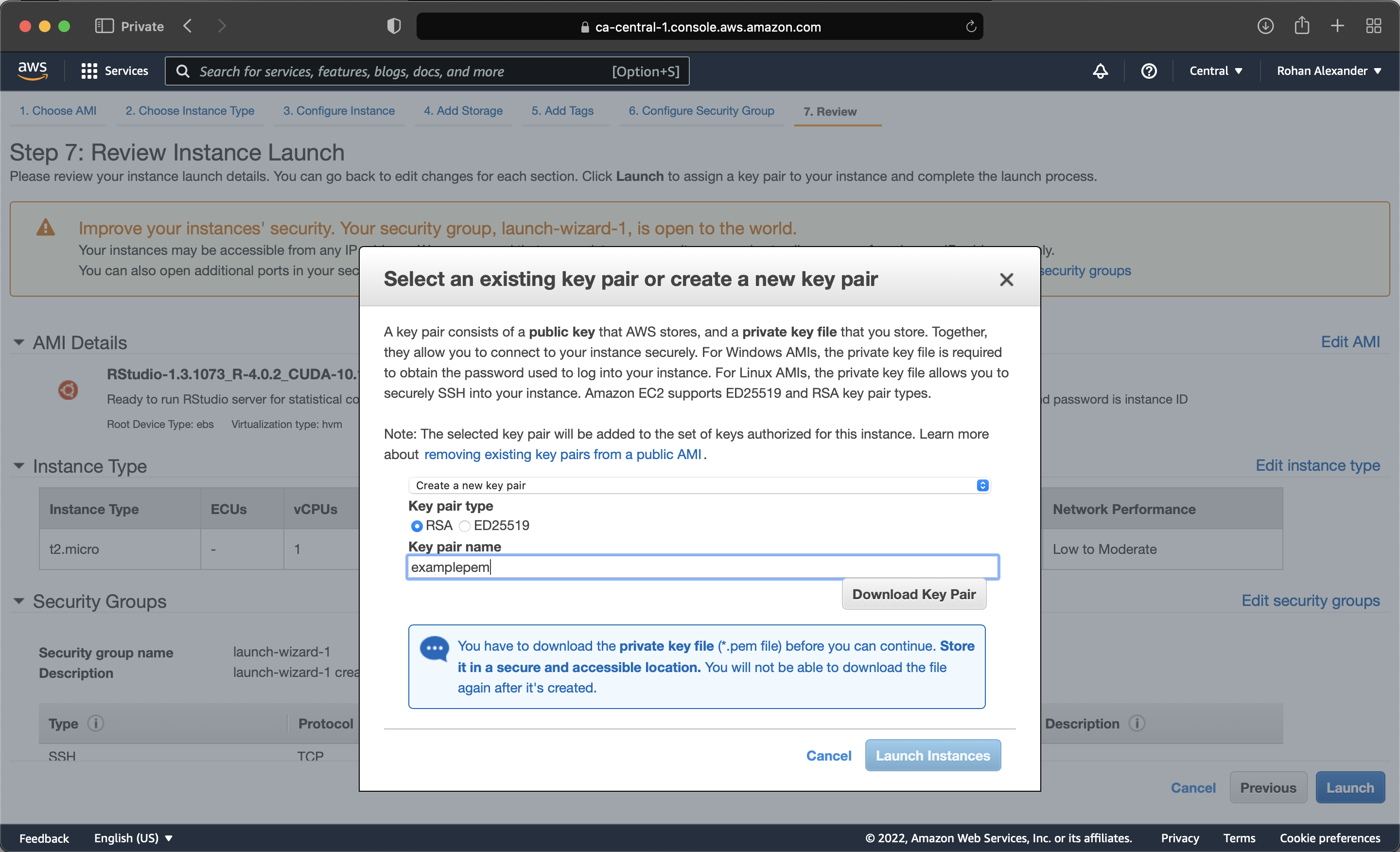
In the next step we can choose how powerful the computer will be. The free tier is a basic computer, but we can choose better ones when we need them. At this point we can pretty much just launch the instance (Figure I.1 (c)). If we start using AWS more seriously, then we could go back and select different options, especially around the security of the account. AWS relies on key pairs. And so, we will need to create a Privacy Enhanced Mail (PEM) and save it locally (Figure I.1 (d)). We can then launch the instance.
After a few minutes, the instance will be running. We can use it by pasting the “public DNS” into a browser. The username is “rstudio” and the password is the instance ID.
We should have RStudio running, which is exciting. The first thing to do is probably to change the default password using the instructions in the instance.
We do not need to install, say, the tidyverse, instead we can just call the library and keep going. This is because this AMI comes with many packages already installed. We can see the list of packages that are installed with installed.packages(). For instance, rstan is already installed, and we could set up an instance with GPUs if we needed.
Perhaps as important as being able to start a AWS instance is being able to stop it (so that we do not get billed). The free tier is useful, but we do need to turn it off. To stop an instance, in the AWS instances page, select it, then “Actions -> Instance State -> Terminate”.
I.3 Plumber and model APIs
The general idea behind the plumber package (Schloerke and Allen 2022) is that we can train a model and make it available via an API that we can call when we want a forecast. Recall in Chapter 7 that we informally defined an API in the context of data gathering as a website that was set-up for another computer to access it, rather than a person. Here, we broaden that to enable data to encompass a model.
Just to get something working, let us make a function that returns “Hello Toronto” regardless of the output. Open a new R file, add the following, and then save it as “plumber.R” (you may need to install the plumber package if you have not done that yet).
#* @get /print_toronto
print_toronto <- function() {
  result <- "Hello Toronto"
  return(result)
}
After that is saved, in the top right of the editor you should get a button to “Run API”. Click that, and your API should load. It will be a “Swagger” application, which provides a GUI around our API. Expand the GET method, and then click “Try it out” and “Execute”. In the response body, you should get “Hello Toronto”.
To more closely reflect the fact that this is an API designed for computers, you can copy/paste the “Request URL” into a browser and it should return “Hello Toronto”.
I.3.0.1 Local model
Now, we are going to update the API so that it serves a model output, given some input. This follows Buhr (2017).
At this point, we should start a new R Project. To get started, let us simulate some data and then train a model on it. In this case we are interested in forecasting how long a baby may sleep overnight, given we know how long they slept during their afternoon nap.
set.seed(853)

number_of_observations <- 1000

baby_sleep <-
  tibble(
    afternoon_nap_length = rnorm(number_of_observations, 120, 5) |> abs(),
    noise = rnorm(number_of_observations, 0, 120),
    night_sleep_length = afternoon_nap_length * 4 + noise,
  )

baby_sleep |>
  ggplot(aes(x = afternoon_nap_length, y = night_sleep_length)) +
  geom_point(alpha = 0.5) +
  labs(
    x = "Baby's afternoon nap length (minutes)",
    y = "Baby's overnight sleep length (minutes)"
  ) +
  theme_classic()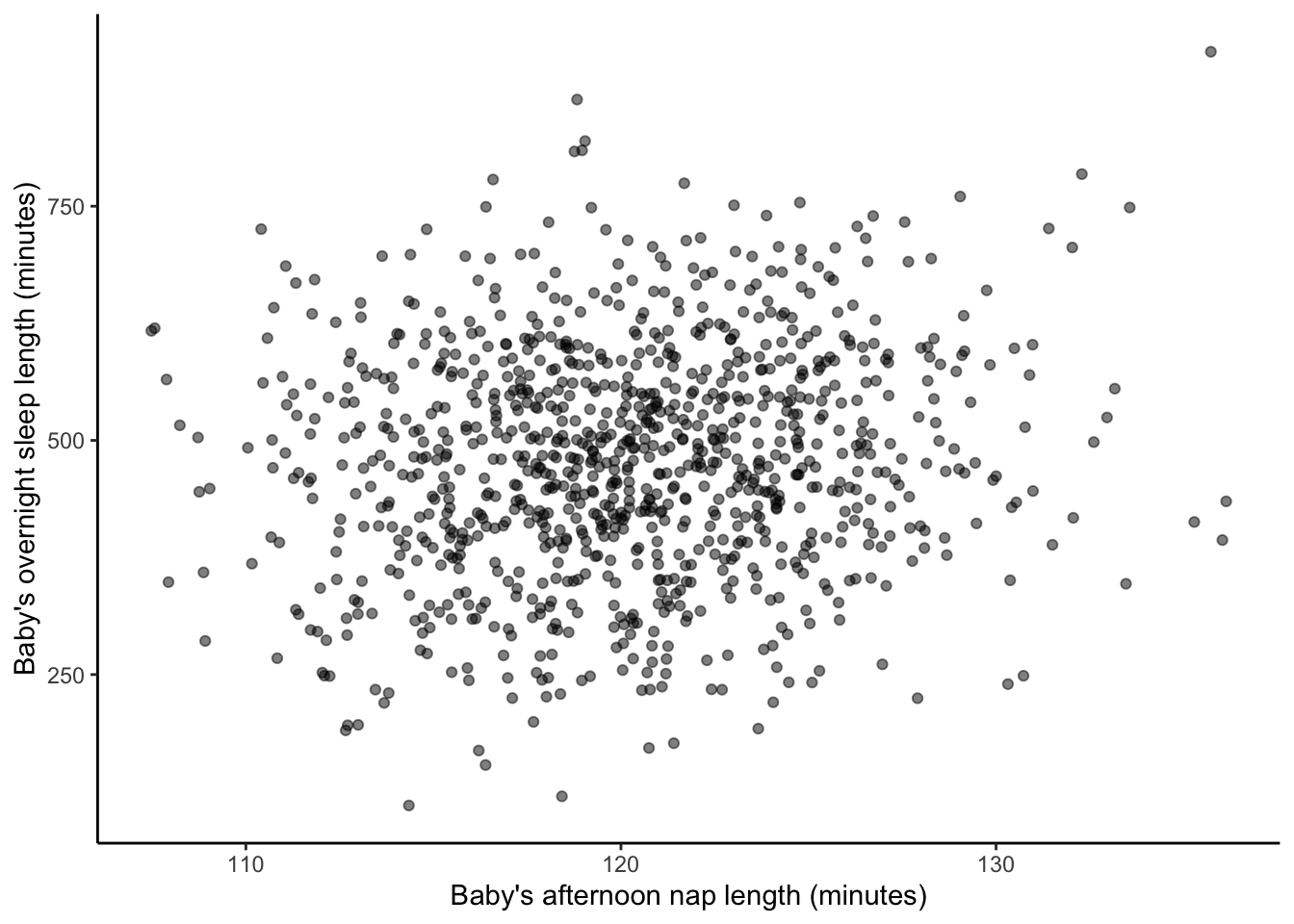
Let us now use tidymodels to quickly make a model.
set.seed(853)

baby_sleep_split <- initial_split(baby_sleep, prop = 0.80)
baby_sleep_train <- training(baby_sleep_split)
baby_sleep_test <- testing(baby_sleep_split)

model <-
  linear_reg() |>
  set_engine(engine = "lm") |>
  fit(
    night_sleep_length ~ afternoon_nap_length,
    data = baby_sleep_train
  )

write_rds(x = model, file = "baby_sleep.rds")
At this point, we have a model. One difference from what you might be used to is that we have saved the model as an “.rds” file. We are going to read that in.
Now that we have our model we want to put that into a file that we will use the API to access, again called “plumber.R”. And we also want a file that sets up the API, called “server.R”. Make an R script called “server.R” and add the following content:
library(plumber)

serve_model <- plumb("plumber.R")
serve_model$run(port = 8000)
Then in “plumber.R” add the following content:
library(plumber)
library(tidyverse)

model <- readRDS("baby_sleep.rds")

version_number <- "0.0.1"

variables <-
  list(
    afternoon_nap_length = "A value in minutes, likely between 0 and 240.",
    night_sleep_length = "A forecast, in minutes, likely between 0 and 1000."
  )

#* @param afternoon_nap_length
#* @get /survival
predict_sleep <- function(afternoon_nap_length = 0) {
  afternoon_nap_length <- as.integer(afternoon_nap_length)

  payload <- data.frame(afternoon_nap_length = afternoon_nap_length)

  prediction <- predict(model, payload)

  result <- list(
    input = list(payload),
    response = list("estimated_night_sleep" = prediction),
    status = 200,
    model_version = version_number
  )

  return(result)
}
Again, after we save the “plumber.R” file we should have an option to “Run API”. Click that and you can try out the API locally in the same way as before. In this case, click “Try It Out” and then input an afternoon nap length in minutes. The response body will contain the prediction based on the data and model we set up.
I.3.0.2 Cloud model
To this point, we have got an API working on our own machine, but what we really want to do is to get it working on a computer such that the API can be accessed by anyone. To do this we are going to use DigitalOcean. It is a charged service, but when you create an account, it will come with $200 in credit, which will be enough to get started.
This set-up process will take some time, but we only need to do it once. Two additional packages that will assist here are plumberDeploy (Allen 2021) and analogsea (Chamberlain et al. 2022) (which will need to be installed from GitHub: install_github("sckott/analogsea")).
Now we need to connect the local computer with the DigitalOcean account.
account()Now we need to authenticate the connection, and this is done using a SSH public key.
key_create()What you want is to have a “.pub” file on our computer. Then copy the public key aspect in that file, and add it to the SSH keys section in the account security settings. When we have the key on our local computer, then we can check this using ssh.
ssh_key_info()Again, this will all take a while to validate. DigitalOcean calls every computer that we start a “droplet”. If we start three computers, then we will have started three droplets. We can check the droplets that are running.
droplets()If everything is set up properly, then this will print the information about all droplets that you have associated with the account (which at this point, is probably none). We must first create a droplet.
id <- do_provision(example = FALSE)Then we get asked for the SSH passphrase and then it will set up a bunch of things. After this we are going to need to install a whole bunch of things onto our droplet.
install_r_package(
  droplet = id,
  c(
    "plumber",
    "remotes",
    "here"
  )
)

debian_apt_get_install(
  id,
  "libssl-dev",
  "libsodium-dev",
  "libcurl4-openssl-dev"
)

debian_apt_get_install(
  id,
  "libxml2-dev"
)

install_r_package(
  id,
  c(
    "config",
    "httr",
    "urltools",
    "plumber"
  )
)

install_r_package(id, c("xml2"))
install_r_package(id, c("tidyverse"))
install_r_package(id, c("tidymodels"))
And then when that is finally set up (it will take 30 minutes or so) we can deploy our API.
do_deploy_api(
  droplet = id,
  path = "example",
  localPath = getwd(),
  port = 8000,
  docs = TRUE,
  overwrite = TRUE
)
I.4 Exercises
Scales
- (Plan)
- (Simulate)
- (Acquire)
- (Explore)
- (Communicate)