library(arrow)
library(devtools)
library(diffpriv)
library(fs)
library(janitor)
library(openssl)
library(tictoc)
library(tidyverse)
library(tinytable)Prerequisites
- Read Promoting Open Science Through Research Data Management, (Borghi and Van Gulick 2022)
- Describes the state of data management, and some strategies for conducting research that is more reproducible.
- Read Data Management in Large-Scale Education Research, (Lewis 2024)
- Focus on Chapter 2 “Research Data Management”, which provides an overview of data management concerns, workflow, and terminology.
- Read Transparent and reproducible social science research, (Christensen, Freese, and Miguel 2019)
- Focus on Chapter 10 “Data Sharing”, which specifies ways to share data.
- Read Datasheets for datasets, (Gebru et al. 2021)
- Introduces the idea of a datasheet.
- Read Data and its (dis)contents: A survey of dataset development and use in machine learning research, (Paullada et al. 2021)
- Details the state of data in machine learning.
Key concepts and skills
- The FAIR principles provide the foundation from which we consider data sharing and storage. These specify that data should be findable, accessible, interoperable, and reusable.
- The most important step is the first one, and that is to get the data off our local computer, and to then make it accessible by others. After that, we build documentation, and datasheets, to make it easier for others to understand and use it. Finally, we ideally enable access without our involvement.
- At the same time as wanting to share our datasets as widely as possible, we should respect those whose information are contained in them. This means, for instance, protecting, to a reasonable extent, and informed by costs and benefits, personally identifying information through selective disclosure, hashing, data simulation, and differential privacy.
- Finally, as our data get larger, approaches that were viable when they were smaller start to break down. We need to consider efficiency, and explore other approaches, formats, and languages.
Software and packages
- Base R (R Core Team 2024)
arrow(Richardson et al. 2023)devtools(Wickham et al. 2022)diffpriv(Rubinstein and Alda 2017)fs(Hester, Wickham, and Csárdi 2021)janitor(Firke 2023)openssl(Ooms 2022)tictoc(Izrailev 2022)tidyverse(Wickham et al. 2019)tinytable(Arel-Bundock 2024)
10.1 Introduction
After we have put together a dataset we must store it appropriately and enable easy retrieval both for ourselves and others. There is no completely agreed on approach, but there are best standards, and this is an evolving area of research (Lewis 2024). Wicherts, Bakker, and Molenaar (2011) found that a reluctance to share data was associated with research papers that had weaker evidence and more potential errors. While it is possible to be especially concerned about this—and entire careers and disciplines are based on the storage and retrieval of data—to a certain extent, the baseline is not onerous. If we can get our dataset off our own computer, then we are much of the way there. Further confirming that someone else can retrieve and use it, ideally without our involvement, puts us much further than most. Just achieving that for our data, models, and code meets the “bronze” standard of Heil et al. (2021).
The FAIR principles are useful when we come to think more formally about data sharing and management. This requires that datasets are (Wilkinson et al. 2016):
- Findable. There is one, unchanging, identifier for the dataset and the dataset has high-quality descriptions and explanations.
- Accessible. Standardized approaches can be used to retrieve the data, and these are open and free, possibly with authentication, and their metadata persist even if the dataset is removed.
- Interoperable. The dataset and its metadata use a broadly-applicable language and vocabulary.
- Reusable. There are extensive descriptions of the dataset and the usage conditions are made clear along with provenance.
One reason for the rise of data science is that humans are at the heart of it. And often the data that we are interested in directly concern humans. This means that there can be tension between sharing a dataset to facilitate reproducibility and maintaining privacy. Medicine developed approaches to this over a long time. And out of that we have seen the Health Insurance Portability and Accountability Act (HIPAA) in the US, the broader General Data Protection Regulation (GDPR) in Europe introduced in 2016, and the California Consumer Privacy Act (CCPA) introduced in 2018, among others.
Our concerns in data science tend to be about personally identifying information. We have a variety of ways to protect especially private information, such as emails and home addresses. For instance, we can hash those variables. Sometimes we may simulate data and distribute that instead of sharing the actual dataset. More recently, approaches based on differential privacy are being implemented, for instance for the US census. The fundamental problem of data privacy is that increased privacy reduces the usefulness of a dataset. The trade-off means the appropriate decision is nuanced and depends on costs and benefits, and we should be especially concerned about differentiated effects on population minorities.
Just because a dataset is FAIR, it is not necessarily an unbiased representation of the world. Further, it is not necessarily fair in the everyday way that word is used, i.e. impartial and honest (Lima et al. 2022). FAIR reflects whether a dataset is appropriately available, not whether it is appropriate.
Finally, in this chapter we consider efficiency. As datasets and code bases get larger it becomes more difficult to deal with them, especially if we want them to be shared. We come to concerns around efficiency, not for its own sake, but to enable us to tell stories that could not otherwise be told. This might mean moving beyond CSV files to formats with other properties, or even using databases, such as Postgres, although even as we do so acknowledging that the simplicity of a CSV, as it is text-based which lends itself to human inspection, can be a useful feature.
10.2 Plan
The storage and retrieval of information is especially connected with libraries, in the traditional sense of a collection of books. These have existed since antiquity and have well-established protocols for deciding what information to store and what to discard, as well as information retrieval. One of the defining aspects of libraries is deliberate curation and organization. The use of a cataloging system ensures that books on similar topics are located close to each other, and there are typically also deliberate plans for ensuring the collection is up to date. This enables information storage and retrieval that is appropriate and efficient.
Data science relies heavily on the internet when it comes to storage and retrieval. Vannevar Bush, the twentieth century engineer, defined a “memex” in 1945 as a device to store books, records, and communications in a way that supplements memory (Bush 1945). The key to it was the indexing, or linking together, of items. We see this concept echoed just four decades later in the proposal by Tim Berners-Lee for hypertext (Berners-Lee 1989). This led to the World Wide Web and defines the way that resources are identified. They are then transported over the internet, using Hypertext Transfer Protocol (HTTP).
At its most fundamental, the internet is about storing and retrieving data. It is based on making various files on a computer available to others. When we consider the storage and retrieval of our datasets we want to especially contemplate for how long they should be stored and for whom (Michener 2015). For instance, if we want some dataset to be available for a decade, and widely available, then it becomes important to store it in open and persistent formats (Hart et al. 2016). But if we are just using a dataset as part of an intermediate step, and we have the original, unedited data and the scripts to create it, then it might be fine to not worry too much about such considerations. The evolution of physical storage media has similar complicated issues. For instance, datasets and recordings made on media such as wax cylinders, magnetic tapes, and proprietary optical disks, now have a variable ease of use.
Storing the original, unedited data is important and there are many cases where unedited data have revealed or hinted at fraud (Simonsohn 2013). Shared data also enhances the credibility of our work, by enabling others to verify it, and can lead to the generation of new knowledge as others use it to answer different questions (Christensen, Freese, and Miguel 2019). Christensen et al. (2019) suggest that research that shares its data may be more highly cited, although Tierney and Ram (2021) caution that widespread data sharing may require a cultural change.
We should try to invite scrutiny and make it as easy as possible to receive criticism. We should try to do this even when it is the difficult choice and results in discomfort because that is the only way to contribute to the stock of lasting knowledge. For instance, Piller (2022) details potential fabrication in research about Alzheimer’s disease. In that case, one of the issues that researchers face when trying to understand whether the results are legitimate is a lack of access to unpublished images.
Data provenance is especially important. This refers to documenting “where a piece of data came from and the process by which it arrived in the database” (Buneman, Khanna, and Wang-Chiew 2001, 316). Documenting and saving the original, unedited dataset, using scripts to manipulate it to create the dataset that is analyzed, and sharing all of this—as recommended in this book—goes some way to achieving this. In some fields it is common for just a handful of databases to be used by many different teams, for instance, in genetics, the UK BioBank, and in the life sciences a cloud-based platform called ORCESTRA (Mammoliti et al. 2021) has been established to help.
10.3 Share
10.3.1 GitHub
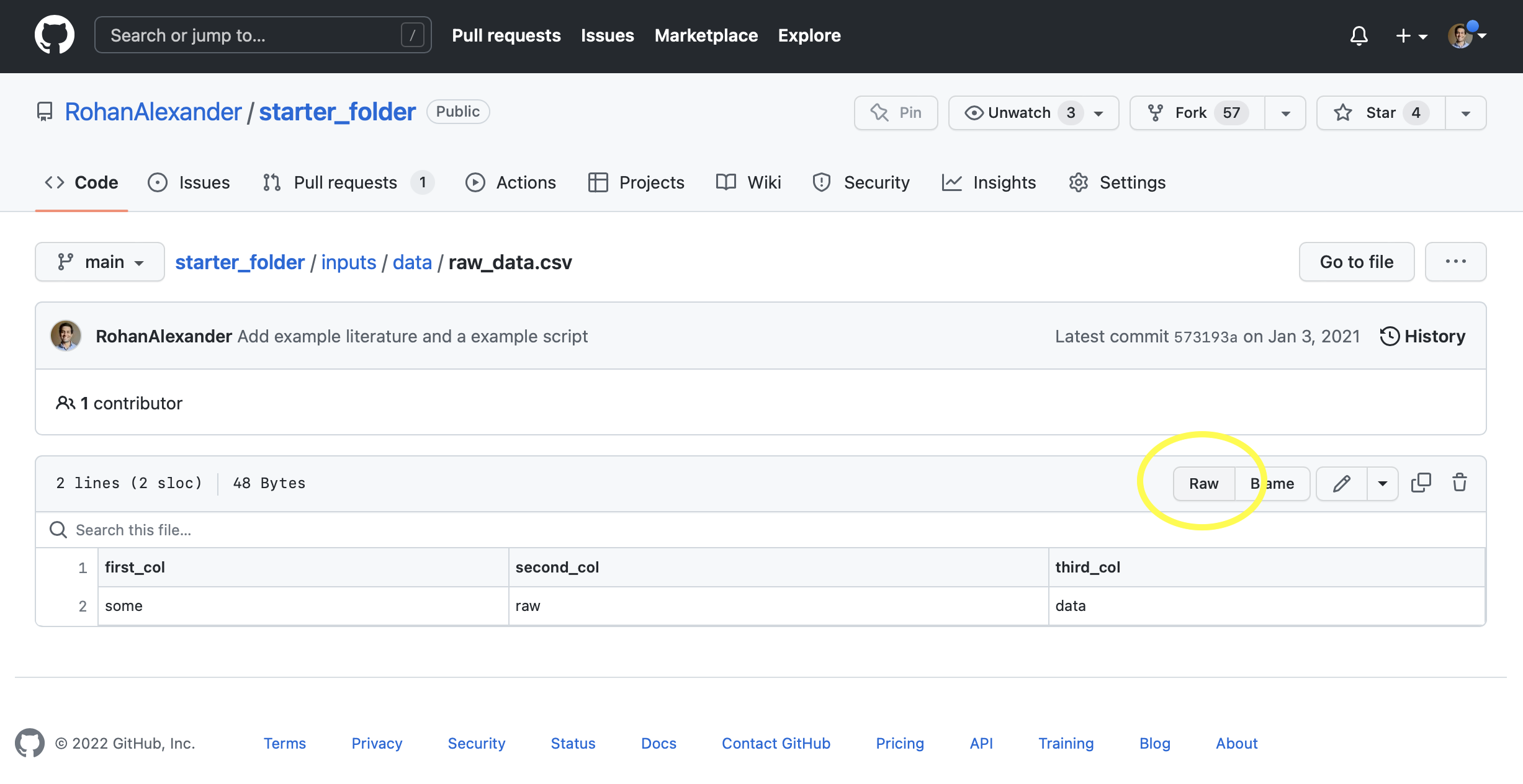
The easiest place for us to get started with storing a dataset is GitHub because that is already built into our workflow. For instance, if we push a dataset to a public repository, then our dataset becomes available. One benefit of this is that if we have set up our workspace appropriately, then we likely store our original, unedited data and the tidy data, as well as the scripts that are needed to transform one to the other. We are most of the way to the “bronze” standard of Heil et al. (2021) without changing anything.
As an example of how we have stored some data, we can access “raw_data.csv” from the “starter_folder”. We navigate to the file in GitHub (“inputs” \(\rightarrow\) “data” \(\rightarrow\) “raw_data.csv”), and then click “Raw” (Figure 10.1).
We can then add that URL as an argument to read_csv().
data_location <-
  paste0(
    "https://raw.githubusercontent.com/RohanAlexander/",
    "starter_folder/main/data/01-raw_data/raw_data.csv"
  )

starter_data <-
  read_csv(file = data_location,
           col_types = cols(
             first_col = col_character(),
             second_col = col_character(),
             third_col = col_character()
             )
           )

starter_data
# A tibble: 1 × 3
first_col second_col third_col
<chr> <chr> <chr>
1 some raw data While we can store and retrieve a dataset easily in this way, it lacks explanation, a formal dictionary, and aspects such as a license that would bring it closer to aligning with the FAIR principles. Another practical concern is that the maximum file size on GitHub is 100MB, although Git Large File Storage (LFS) can be used if needed. And a final concern, for some, is that GitHub is owned by Microsoft, a for-profit US technology firm.
10.3.2 R packages for data
To this point we have largely used R packages for their code, although we have seen a few that were focused on sharing data, for instance, troopdata and babynames in Chapter 5. We can build a R package for our dataset and then add it to GitHub and potentially eventually CRAN. This will make it easy to store and retrieve because we can obtain the dataset by loading the package. In contrast to the CSV-based approach, it also means a dataset brings its documentation along with it.
This will be the first R package that we build, and so we will jump over a number of steps. The key is to just try to get something working. In Appendix G, we return to R packages and use them to deploy models. This gives us another chance to further develop experience with them.
To get started, create a new package: “File” \(\rightarrow\) “New project” \(\rightarrow\) “New Directory” \(\rightarrow\) “R Package”. Give the package a name, such as “favcolordata” and select “Open in new session”. Create a new folder called “data”. We will simulate a dataset of people and their favorite colors to include in our R package.
set.seed(853)

color_data <-
  tibble(
    name =
      c(
        "Edward", "Helen", "Hugo", "Ian", "Monica",
        "Myles", "Patricia", "Roger", "Rohan", "Ruth"
      ),
    fav_color =
      sample(
        x = colors(),
        size = 10,
        replace = TRUE
      )
  )
To this point we have largely been using CSV files for our datasets. To include our data in this R package, we save our dataset in a different format, “.rda”, using save().
save(color_data, file = "data/color_data.rda")Then we create a R file “data.R” in the “R” folder. This file will only contain documentation using roxygen2 comments. These start with #', and we follow the documentation for troopdata closely.
#' Favorite color of various people data
#'
#' @description \code{favcolordata} returns a dataframe
#' of the favorite color of various people.
#'
#' @return Returns a dataframe of the favorite color
#' of various people.
#'
#' @docType data
#'
#' @usage data(color_data)
#'
#' @format A dataframe of individual-level observations
#' with the following variables:
#'
#' \describe{
#' \item{\code{name}}{A character vector of individual names.}
#' \item{\code{fav_color}}{A character vector of colors.}
#' }
#'
#' @keywords datasets
#'
#' @source \url{tellingstorieswithdata.com/10-store_and_share.html}
#'
"color_data"
Finally, add a README that provides a summary of all of this for someone coming to the project for the first time. Examples of packages with excellent READMEs include ggplot2, pointblank, modelsummary, and janitor.
We can now go to the “Build” tab and click “Install and Restart”. After this, the package “favcolordata”, will be loaded and the data can be accessed locally using “color_data”. If we were to push this package to GitHub, then anyone would be able to install the package using devtools and use our dataset. Indeed, the following should work.
install_github("RohanAlexander/favcolordata")

library(favcolordata)

color_data
This has addressed many of the issues that we faced earlier. For instance, we have included a README and a data dictionary, of sorts, in terms of the descriptions that we added. But if we were to try to put this package onto CRAN, then we might face some issues. For instance, the maximum size of a package is 5MB and we would quickly come up against that. We have also largely forced users to use R. While there are benefits of that, we may like to be more language agnostic (Tierney and Ram 2020), especially if we are concerned about the FAIR principles.
Wickham (2022, chap. 8) provides more information about including data in R packages.
10.3.3 Depositing data
While it is possible that a dataset will be cited if it is available through GitHub or a R package, this becomes more likely if the dataset is deposited somewhere. There are several reasons for this, but one is that it seems a bit more formal. Another is that it is associated with a DOI. Zenodo and the Open Science Framework (OSF) are two depositories that are commonly used. For instance, Carleton (2021) uses Zenodo to share the dataset and analysis supporting Carleton, Campbell, and Collard (2021), Geuenich et al. (2021b) use Zenodo to share the dataset that underpins Geuenich et al. (2021a), and Katz and Alexander (2023a) use Zenodo to share the dataset that underpins Katz and Alexander (2023b). Similarly, Arel-Bundock et al. (2022) use OSF to share code and data.
Another option is to use a dataverse, such as the Harvard Dataverse or the Australian Data Archive. This is a common requirement for journal publications. One nice aspect of this is that we can use dataverse to retrieve the dataset as part of a reproducible workflow. We have an example of this in Chapter 13.
In general, these options are free and provide a DOI that can be useful for citation purposes. The use of data deposits such as these is a way to offload responsibility for the continued hosting of the dataset (which in this case is a good thing) and prevent the dataset from being lost. It also establishes a single point of truth, which should act to reduce errors (Byrd et al. 2020). Finally, it makes access to the dataset independent of the original researchers, and results in persistent metadata. That all being said, the viability of these options rests on their underlying institutions. For instance, Zenodo is operated by CERN and many dataverses are operated by universities. These institutions are subject to, as we all are, social and political forces.
10.4 Data documentation
Dataset documentation has long consisted of a data dictionary. This may be as straight-forward a list of the variables, a few sentences of description, and ideally a source. The data dictionary of the ACS, which was introduced in Chapter 6, is particularly comprehensive. And OSF provides instructions for how to make a data dictionary. Given the workflow advocated in this book, it might be worthwhile to actually begin putting together a data dictionary as part of the simulation step i.e. before even collecting the data. While it would need to be updated, it would be another opportunity to think deeply about the data situation.
Datasheets (Gebru et al. 2021) are an increasingly common addition to documentation. If we think of a data dictionary as a list of ingredients for a dataset, then we could think of a datasheet as basically a nutrition label for datasets. The process of creating them enables us to think more carefully about what we will feed our model. More importantly, they enable others to better understand what we fed our model. One important task is going back and putting together datasheets for datasets that are widely used. For instance, researchers went back and wrote a datasheet for “BookCorpus”, which is one of the most popular datasets in computer science, and they found that around 30 per cent of the data were duplicated (Bandy and Vincent 2021).
Shoulders of giants
Timnit Gebru is the founder of the Distributed Artificial Intelligence Research Institute (DAIR). After earning a PhD in Computer Science from Stanford University, Gebru joined Microsoft and then Google. In addition to Bandy and Vincent (2021), which introduced datasheets, one notable paper is Bender et al. (2021), which discussed the dangers of language models being too large. She has made many other substantial contributions to fairness and accountability, especially Buolamwini and Gebru (2018), which demonstrated racial bias in facial analysis algorithms.
Instead of telling us how unhealthy various foods are, a datasheet tells us things like:
- Who put the dataset together?
- Who paid for the dataset to be created?
- How complete is the dataset? (Which is, of course, unanswerable, but detailing the ways in which it is known to be incomplete is valuable.)
- Which variables are present, and, equally, not present, for particular observations?
Sometimes, a lot of work is done to create a datasheet. In that case, we may like to publish and share it on its own, for instance, Biderman, Bicheno, and Gao (2022) and Bandy and Vincent (2021). But typically a datasheet might live in an appendix to the paper, for instance Zhang et al. (2022), or be included in a file adjacent to the dataset.
When creating a datasheet for a dataset, especially a dataset that we did not put together ourselves, it is possible that the answer to some questions will simply be “Unknown”, but we should do what we can to minimize that. The datasheet template created by Gebru et al. (2021) is not the final word. It is possible to improve on it, and add additional detail sometimes. For instance, Miceli, Posada, and Yang (2022) argue for the addition of questions to do with power relations.
10.5 Personally identifying information
By way of background, Christensen, Freese, and Miguel (2019, 180) define a variable as “confidential” if the researchers know who is associated with each observation, but the public version of the dataset removes this association. A variable is “anonymous” if even the researchers do not know.
Personally identifying information (PII) is that which enables us to link an observation in our dataset with an actual person. This is a significant concern in fields focused on data about people. Email addresses are often PII, as are names and addresses. While some variables may not be PII for many respondents, it could be PII for some. For instance, consider a survey that is representative of the population age distribution. There is not likely to be many respondents aged over 100, and so the variable age may then become PII. The same scenario applies to income, wealth, and many other variables. One response to this is for data to be censored, which was discussed in Chapter 6. For instance, we may record age between zero and 90, and then group everyone over that into “90+”. Another is to construct age-groups: “18-29”, “30-44”, \(\dots\). Notice that with both these solutions we have had to trade-off privacy and usefulness. More concerningly, a variable may be PII, not by itself, but when combined with another variable.
Our primary concern should be with ensuring that the privacy of our dataset is appropriate, given the expectations of the reasonable person. This requires weighing costs and benefits. In national security settings there has been considerable concern about the over-classification of documents (Lin 2014). The reduced circulation of information because of this may result in unrealized benefits. To avoid this in data science, the test of the need to protect a dataset needs to be made by the reasonable person weighing up costs and benefits. It is easy, but incorrect, to argue that data should not be released unless it is perfectly anonymized. The fundamental problem of data privacy implies that such data would have limited utility. That approach, possibly motivated by the precautionary principle, would be too conservative and could cause considerable loss in terms of unrealized benefits.
Randomized response (Greenberg et al. 1969) is a clever way to enable anonymity without much overhead. Each respondent flips a coin before they answer a question but does not show the researcher the outcome of the coin flip. The respondent is instructed to respond truthfully to the question if the coin lands on heads, but to always give some particular (but still plausible) response if tails. The results of the other options can then be re-weighted to enable an estimate, without a researcher ever knowing the truth about any particular respondent. This is especially used in association with snowball sampling, discussed in Chapter 6. One issue with randomized response is that the resulting dataset can be only used to answer specific questions. This requires careful planning, and the dataset will be of less general value.
Zook et al. (2017) recommend considering whether data even need to be gathered in the first place. For instance, if a phone number is not absolutely required then it might be better to not ask for it, rather than need to worry about protecting it before data dissemination. GDPR and HIPAA are two legal structures that govern data in Europe, and the United States, respectively. Due to the influence of these regions, they have a significant effect outside those regions also. GDPR concerns data generally, while HIPAA is focused on healthcare. GDPR applies to all personal data, which is defined as:
\(\dots\)any information relating to an identified or identifiable natural person (“data subject”); an identifiable natural person is one who can be identified, directly or indirectly, in particular by reference to an identifier such as a name, an identification number, location data, an online identifier or to one or more factors specific to the physical, physiological, genetic, mental, economic, cultural or social identity of that natural person;
Council of European Union (2016), Article 4, “Definitions”
HIPAA refers to the privacy of medical records in the US and codifies the idea that the patient should have access to their medical records, and that only the patient should be able to authorize access to their medical records (Annas 2003). HIPAA only applies to certain entities. This means it sets a standard, but coverage is inconsistent. For instance, a person’s social media posts about their health would generally not be subject to it, nor would knowledge of a person’s location and how active they are, even though based on that information we may be able to get some idea of their health (Cohen and Mello 2018). Such data are hugely valuable (Ross 2022).
There are a variety of ways of protecting PII, while still sharing some data, that we will now go through. We focus here initially on what we can do when the dataset is considered by itself, which is the main concern. But sometimes the combination of several variables, none of which are PII in and of themselves, can be PII. For instance, age is unlikely PII by itself, but age combined with city, education, and a few other variables could be. One concern is that re-identification could occur by combining datasets and this is a potential role for differential privacy.
10.5.1 Hashing
A cryptographic hash is a one-way transformation, such that the same input always provides the same output, but given the output, it is not reasonably possible to obtain the input. For instance, a function that doubled its input always gives the same output, for the same input, but is also easy to reverse, so would not work well as a hash. In contrast, the modulo, which for a non-negative number is the remainder after division and can be implemented in R using %%, would be difficult to reverse.
Knuth (1998, 514) relates an interesting etymology for “hash”. He first defines “to hash” as relating to chop up or make a mess, and then explaining that hashing relates to scrambling the input and using this partial information to define the output. A collision is when different inputs map to the same output, and one feature of a good hashing algorithm is that collisions are reduced. As mentioned, one simple approach is to rely on the modulo operator. For instance, if we were interested in ten different groupings for the integers 1 through to 10, then modulo would enable this. A better approach would be for the number of groupings to be a larger number, because this would reduce the number of values with the same hash outcome.
For instance, consider some information that we would like to keep private, such as names and ages of respondents.
some_private_information <-
  tibble(
    names = c("Rohan", "Monica"),
    ages = c(36, 35)
  )

some_private_information
# A tibble: 2 × 2
names ages
<chr> <dbl>
1 Rohan 36
2 Monica 35One option for the names would be to use a function that just took the first letter of each name. And one option for the ages would be to convert them to Roman numerals.
some_private_information |>
  mutate(
    names = substring(names, 1, 1),
    ages = as.roman(ages)
  )
# A tibble: 2 × 2
names ages
<chr> <roman>
1 R XXXVI
2 M XXXV While the approach for the first variable, names, is good because the names cannot be backed out, the issue is that as the dataset grows there are likely to be lots of “collisions”—situations where different inputs, say “Rohan” and “Robert”, both get the same output, in this case “R”. It is the opposite situation for the approach for the second variable, ages. In this case, there will never be any collisions—“36” will be the only input that ever maps to “XXXVI”. However, it is easy to back out the actual data, for anyone who knows roman numerals.
Rather than write our own hash functions, we can use cryptographic hash functions such as md5() from openssl.
some_private_information |>
  mutate(
    md5_names = md5(names),
    md5_ages = md5(ages |> as.character())
  )
# A tibble: 2 × 4
names ages md5_names md5_ages
<chr> <dbl> <hash> <hash>
1 Rohan 36 02df8936eee3d4d2568857ed530671b2 19ca14e7ea6328a42e0eb13d585e4c22
2 Monica 35 09084cc0cda34fd80bfa3cc0ae8fe3dc 1c383cd30b7c298ab50293adfecb7b18We could share either of these transformed variables and be comfortable that it would be difficult for someone to use only that information to recover the names of our respondents. That is not to say that it is impossible. Knowledge of the key, which is the term given to the string used to encrypt the data, would allow someone to reverse this. If we made a mistake, such as accidentally pushing the original dataset to GitHub then they could be recovered. And it is likely that governments and some private companies can reverse the cryptographic hashes used here.
One issue that remains is that anyone can take advantage of the key feature of hashes to back out the input. In particular, the same input always gets the same output. So they could test various options for inputs. For instance, they could themselves try to hash “Rohan”, and then noticing that the hash is the same as the one that we published in our dataset, know that data relates to that individual. We could try to keep our hashing approach secret, but that is difficult as there are only a few that are widely used. One approach is to add a salt that we keep secret. This slightly changes the input. For instance, we could add the salt “_is_a_person” to all our names and then hash that, although a large random number might be a better option. Provided the salt is not shared, then it would be difficult for most people to reverse our approach in that way.
some_private_information |>
  mutate(names = paste0(names, "_is_a_person")) |>
  mutate(
    md5_of_salt = md5(names)
  )
# A tibble: 2 × 3
names ages md5_of_salt
<chr> <dbl> <hash>
1 Rohan_is_a_person 36 3ab064d7f746fde604122d072fd4fa97
2 Monica_is_a_person 35 50bb9dfffa926c855b830845ac61b65910.5.2 Simulation
One common approach to deal with the issue of being unable to share the actual data that underpins an analysis, is to use data simulation. We have used data simulation throughout this book toward the start of the workflow to help us to think more deeply about our dataset. We can use data simulation again at the end, to ensure that others cannot access the actual dataset.
The approach is to understand the critical features of the dataset and the appropriate distribution. For instance, if our data were the ages of some population, then we may want to use the Poisson distribution and experiment with different parameters for the rate. Having simulated a dataset, we conduct our analysis using this simulated dataset and ensure that the results are broadly similar to when we use the real data. We can then release the simulated dataset along with our code.
For more nuanced situations, Koenecke and Varian (2020) recommend using the synthetic data vault (Patki, Wedge, and Veeramachaneni 2016) and then the use of Generative Adversarial Networks, such as implemented by Athey et al. (2021).
10.5.3 Differential privacy
Differential privacy is a mathematical definition of privacy (Dwork and Roth 2013, 6). It is not just one algorithm, it is a definition that many algorithms satisfy. Further, there are many definitions of privacy, of which differential privacy is just one. The main issue it solves is that there are many datasets available. This means there is always the possibility that some combination of them could be used to identify respondents even if PII were removed from each of these individual datasets. For instance, experience with the Netflix prize found that augmenting the available dataset with data from IMBD resulted in better predictions, which points to why this would so commonly happen. Rather than needing to anticipate how various datasets could be combined to re-identify individuals and adjust variables to remove this possibility, a dataset that is created using a differentially private approach provides assurances that privacy will be maintained.
Shoulders of giants
Cynthia Dwork is the Gordon McKay Professor of Computer Science at Harvard University. After earning a PhD in Computer Science from Cornell University, she was a Post-Doctoral Research Fellow at MIT and then worked at IBM, Compaq, and Microsoft Research where she is a Distinguished Scientist. She joined Harvard in 2017. One of her major contributions is differential privacy (Dwork et al. 2006), which has become widely used.
To motivate the definition, consider a dataset of responses and PII that only has one person in it. The release of that dataset, as is, would perfectly identify them. At the other end of the scale, consider a dataset that does not contain a particular person. The release of that dataset could, in general, never be linked to them because they are not in it.1 Differential privacy, then, is about the inclusion or exclusion of particular individuals in a dataset. An algorithm is differentially private if the inclusion or exclusion of any particular person in a dataset has at most some given factor of an effect on the probability of some output (Oberski and Kreuter 2020). The fundamental problem of data privacy is that we cannot have completely anonymized data that remains useful (Dwork and Roth 2013, 6). Instead, we must trade-off utility and privacy.
A dataset is differentially private to different levels of privacy, based on how much it changes when one person’s results are included or excluded. This is the key parameter, because at the same time as deciding how much of an individual’s information we are prepared to give up, we are deciding how much random noise to add, which will impact our output. The choice of this level is a nuanced one and should involve consideration of the costs of undesired disclosures, compared with the benefits of additional research. For public data that will be released under differential privacy, the reasons for the decision should be public because of the costs that are being imposed. Indeed, Tang et al. (2017) argue that even in the case of private companies that use differential privacy, such as Apple, users should have a choice about the level of privacy loss.
Consider a situation in which a professor wants to release the average mark for a particular assignment. The professor wants to ensure that despite that information, no student can work out the grade that another student got. For instance, consider a small class with the following marks.
set.seed(853)

grades <-
  tibble(ps_1 = sample(x = (1:100), size = 10, replace = TRUE))

mean(grades$ps_1)
[1] 50.5The professor could announce the exact mean, for instance, “The mean for the first problem set was 50.5”. Theoretically, all-but-one student could let the others know their mark. It would then be possible for that group to determine the mark of the student who did not agree to make their mark public.
A non-statistical approach would be for the professor to add the word “roughly”. For instance, the professor could say “The mean for the first problem set was roughly 50.5”. The students could attempt the same strategy, but they would never know with certainty. The professor could implement a more statistical approach to this by adding noise to the mean.
mean(grades$ps_1) + runif(n = 1, min = -2, max = 2)[1] 48.91519The professor could then announce this modified mean. This would make the students’ plan more difficult. One thing to notice about that approach is that it would not work with persistent questioning. For instance, eventually the students would be able to back out the distribution of the noise that the professor added. One implication is that the professor would need to limit the number of queries they answered about the mean of the problem set.
A differentially private approach is a sophisticated version of this. We can implement it using diffpriv. This results in a mean that we could announce (Table 10.1).
# Code based on the diffpriv example
target <- function(X) mean(X)

mech <- DPMechLaplace(target = target)

distr <- function(n) rnorm(n)

mech <- sensitivitySampler(mech, oracle = distr, n = 5, gamma = 0.1)

r <- releaseResponse(mech,
                     privacyParams = DPParamsEps(epsilon = 1),
X = grades$ps_1)| Actual mean | Announceable mean |
|---|---|
| 50.5 | 52.5 |
The implementation of differential privacy is a costs and benefits issue (Hotz et al. 2022; Kenny et al. 2023). Stronger privacy protection fundamentally must mean less information (Bowen 2022, 39), and this differently affects various aspects of society. For instance, Suriyakumar et al. (2021) found that, in the context of health care, differentially private learning can result in models that are disproportionately affected by large demographic groups. A variant of differential privacy has recently been implemented by the US census. It may have a significant effect on redistricting (Kenny et al. 2021) and result in some publicly available data that are unusable in the social sciences (Ruggles et al. 2019).
10.6 Data efficiency
For the most part, done is better than perfect, and unnecessary optimization is a waste of resources. However, at a certain point, we need to adapt new ways of dealing with data, especially as our datasets start to get larger. Here we discuss iterating through multiple files, and then turn to the use of Apache Arrow and parquet. Another natural step would be the use of SQL, which is covered in Online Appendix C.
10.6.1 Iteration
There are several ways to become more efficient with our data, especially as it becomes larger. The first, and most obvious, is to break larger datasets into smaller pieces. For instance, if we have a dataset for a year, then we could break it into months, or even days. To enable this, we need a way of quickly reading in many different files.
The need to read in multiple files and combine them into the one tibble is a surprisingly common task. For instance, it may be that the data for a year, are saved into individual CSV files for each month. We can use purrr and fs to do this. To illustrate this situation we will simulate data from the exponential distribution using rexp(). Such data may reflect, say, comments on a social media platform, where the vast majority of comments are made by a tiny minority of users. We will use dir_create() from fs to create a folder, simulate monthly data, and save it. We will then illustrate reading it in.
dir_create(path = "user_data")

set.seed(853)

simulate_and_save_data <- function(month) {
  num_obs <- 1000
  file_name <- paste0("user_data/", month, ".csv")
  user_comments <-
    tibble(
      user = c(1:num_obs),
      month = rep(x = month, times = num_obs),
      comments = rexp(n = num_obs, rate = 0.3) |> round()
    )
  write_csv(
    x = user_comments,
    file = file_name
  )
}

walk(month.name |> tolower(), simulate_and_save_data)
Having created our dataset with each month saved to a different CSV, we can now read it in. There are a variety of ways to do this. The first step is that we need to get a list of all the CSV files in the directory. We use the “glob” argument here to specify that we are interested only in the “.csv” files, and that could change to whatever files it is that we are interested in.
files_of_interest <-
  dir_ls(path = "user_data/", glob = "*.csv")

files_of_interest
[1] "april.csv" "august.csv" "december.csv" "february.csv"
[5] "january.csv" "july.csv" "june.csv" "march.csv"
[9] "may.csv" "november.csv" "october.csv" "september.csv"We can pass this list to read_csv() and it will read them in and combine them.
year_of_data <-
  read_csv(
    files_of_interest,
    col_types = cols(
      user = col_double(),
      month = col_character(),
      comments = col_double(),
    )
  )

year_of_data
# A tibble: 12,000 × 3
user month comments
<dbl> <chr> <dbl>
1 1 april 0
2 2 april 2
3 3 april 2
4 4 april 5
5 5 april 1
6 6 april 3
7 7 april 2
8 8 april 1
9 9 april 4
10 10 april 3
# ℹ 11,990 more rowsIt prints out the first ten days of April, because alphabetically April is the first month of the year and so that was the first CSV that was read.
This works well when we have CSV files, but we might not always have CSV files and so will need another way, and can use map_dfr() to do this. One nice aspect of this approach is that we can include the name of the file alongside the observation using “.id”. Here we specify that we would like that column to be called “file”, but it could be anything.
year_of_data_using_purrr <-
  files_of_interest |>
  map_dfr(read_csv, .id = "file")
# A tibble: 12,000 × 4
file user month comments
<chr> <dbl> <chr> <dbl>
1 april.csv 1 april 0
2 april.csv 2 april 2
3 april.csv 3 april 2
4 april.csv 4 april 5
5 april.csv 5 april 1
6 april.csv 6 april 3
7 april.csv 7 april 2
8 april.csv 8 april 1
9 april.csv 9 april 4
10 april.csv 10 april 3
# ℹ 11,990 more rows10.6.2 Apache Arrow
CSVs are commonly used without much thought in data science. And while CSVs are good because they have little overhead and can be manually inspected, this also means they are quite minimal. This can lead to issues, for instance class is not preserved, and file sizes can become large leading to storage and performance issues. There are various alternatives, including Apache Arrow, which stores data in columns rather than rows like CSV. We focus on the “.parquet” format from Apache Arrow. Like a CSV, parquet is an open standard. The R package, arrow, enables us to use this format. The use of parquet has the advantage of requiring little change from us while delivering significant benefits.
Shoulders of giants
Wes McKinney holds an undergraduate degree in theoretical mathematics from MIT. Starting in 2008, while working at AQR Capital Management, he developed the Python package, pandas, which has become a cornerstone of data science. He later wrote Python for Data Analysis (McKinney [2011] 2022). In 2016, with Hadley Wickham, he designed Feather, which was released in 2016. He now works as CTO of Voltron Data, which focuses on the Apache Arrow project.
In particular, we focus on the benefit of using parquet for data storage, such as when we want to save a copy of an analysis dataset that we cleaned and prepared. Among other aspects, parquet brings two specific benefits, compared with CSV:
- the file sizes are typically smaller; and
- class is preserved because parquet attaches a schema, which makes dealing with, say, dates and factors considerably easier.
Having loaded arrow, we can use parquet files in a similar way to CSV files. Anywhere in our code that we used write_csv() and read_csv() we could alternatively, or additionally, use write_parquet() and read_parquet(), respectively. The decision to use parquet needs to consider both costs and benefits, and it is an active area of development.
num_draws <- 1000000

# Homage: https://www.rand.org/pubs/monograph_reports/MR1418.html
a_million_random_digits <-
  tibble(
    numbers = runif(n = num_draws),
    letters = sample(x = letters, size = num_draws, replace = TRUE),
    states = sample(x = state.name, size = num_draws, replace = TRUE),
  )

write_csv(x = a_million_random_digits,
          file = "a_million_random_digits.csv")

write_parquet(x = a_million_random_digits,
              sink = "a_million_random_digits.parquet")

file_size("a_million_random_digits.csv")29.3Mfile_size("a_million_random_digits.parquet")8.17MWe can write a parquet file with write_parquet() and we can read a parquet with read_parquet(). We get significant reductions in file size when we compare the size of the same datasets saved in each format, especially as they get larger (Table 10.2). The speed benefits of using parquet are most notable for larger datasets. It turns them from being impractical to being usable.
| Number | CSV size | CSV write time (sec) | CSV read time (sec) | Parquet size | Parquet write time (sec) | Parquet read time (sec) |
|---|---|---|---|---|---|---|
| 1e+02 | 3,102.72 | 0.01 | 0.26 | 2,713.6 | 0.01 | 0 |
| 1e+03 | 30,720 | 0.02 | 0.27 | 11,366.4 | 0.01 | 0 |
| 1e+04 | 307,415.04 | 0.02 | 0.3 | 101,969.92 | 0.01 | 0.01 |
| 1e+05 | 3,072,327.68 | 0.03 | 0.28 | 1,040,885.76 | 0.04 | 0.01 |
| 1e+06 | 30,712,791.04 | 0.15 | 0.58 | 8,566,865.92 | 0.22 | 0.05 |
| 1e+07 | 307,117,424.64 | 1 | 2.95 | 82,952,847.36 | 1.76 | 0.42 |
| 1e+08 | 3,070,901,616.64 | 7.65 | 32.89 | 827,137,720.32 | 16.12 | 4.85 |
Crane, Hazlitt, and Arrow (2023) provides further information about specific tasks, Navarro (2022) provides helpful examples of implementation, and Navarro, Keane, and Hazlitt (2022) provides an extensive set of materials. There is no settled consensus on whether parquet files should be used exclusively for dataset. But it is indisputable that the persistence of class alone provides a compelling reason for including them in addition to a CSV.
We will use parquet more in the remainder of this book.
10.7 Exercises
Practice
- (Plan) Consider the following scenario: You work for a large news media company and focus on subscriber management. Over the course of a year most subscribers will never post a comment beneath a news article, but a few post an awful lot. Please sketch what that dataset could look like and then sketch a graph that you could build to show all observations.
- (Simulate) Please further consider the scenario described and simulate the situation. Carefully pick an appropriate distribution. Please include five tests based on the simulated data. Submit a link to a GitHub Gist that contains your code.
- (Acquire) Please describe one possible source of such a dataset.
- (Explore) Please use
ggplot2to build the graph that you sketched. Submit a link to a GitHub Gist that contains your code. - (Communicate) Please write two paragraphs about what you did.
Quiz
- Following Wilkinson et al. (2016), please discuss the FAIR principles in the context of a dataset that you are familiar with (begin with a one-paragraph summary of the dataset, then write one paragraph per principle).
- Please create a R package for a simulated dataset, push it to GitHub, and submit code to install the package (e.g.
devtools::install_github("RohanAlexander/favcolordata")). - According to Gebru et al. (2021), a datasheet should document a dataset’s (please select all that apply):
- composition.
- recommended uses.
- motivation.
- collection process.
- Discuss, with the help of examples and references, whether a person’s name is PII (please write at least three paragraphs)?
- Using
md5()what is the hash of “Monica” (pick one)?- 243f63354f4c1cc25d50f6269b844369
- 02df8936eee3d4d2568857ed530671b2
- 09084cc0cda34fd80bfa3cc0ae8fe3dc
- 1b3840b0b70d91c17e70014c8537dbba
- Please save the
penguinsdata from frompalmerpenguinsas a CSV file and as a Parquet file. How big are they?- 12.5K; 6.04K
- 14.9K; 6.04K
- 14.9K; 5.02K
- 12.5K; 5.02K
Class activities
- Use the starter folder and create a new repo. Add a link to the GitHub repo in the class’s shared Google Doc.
- Add the following code to a simulation R script, then lint it. What do you think about the recommendations?
set.seed(853)
tibble(
  age_days=runif(n=10,min=0,max=36500),
  age_years=age_days%/%365
)- Simulate a dataset with ten million observations and at least five variables, one of which must be a date. Save it in both CSV and parquet formats. What is the file size difference?
- Discuss datasheets in the context of the dataset that you simulated.
- Pretend you were joining two datasets with
left_join(). When joining datasets it is easy to accidentally duplicate or remove rows. Please add some tests that might put your mind at ease.
set.seed(853)

# CONSIDER A CHANGE HERE

main_data <-
  tibble(
    participant_id = stringi::stri_rand_strings(n = 100, length = 5),
    education_value = sample(
      x = 1:5,
      size = 100,
      replace = TRUE
    )
  )

# CONSIDER A CHANGE HERE

education_labels <-
  tibble(
    education_value = 1:5,
    education_label = c(
      "Some high school",
      "High school",
      "Some post secondary",
      "Post secondary degree",
      "Graduate degree"
    )
  )

# CONSIDER A CHANGE HERE

joined_data <-
  main_data |>
  left_join(education_labels, by = join_by(education_value))

# CONSIDER A CHANGE HERE- Modify the following code to show why using “T” instead of “TRUE” should generally not be done (hint: assign “T” to “FALSE”)?
set.seed(853)
# MAKE CHANGE HERE
sample(x = 1:5, size = 5, replace = T)
[1] 1 2 5 1 5- Working with the instructor, pick a chapter from Lewis (2024) and create a five-slide summary of the key take-aways from the chapter. Present to the class.
- Working with the instructor, make a pull request that fixes some small aspect of a work-in-progress book.2 Options include:3 Lewis (2024) or Wickham, Çetinkaya-Rundel, and Grolemund ([2016] 2023).
- Pretend that you are in a small class, and have some results from an assessment (Table 10.3). Use the code, but change the seed to generate your own dataset.
- Hash, but do not salt, the names, and then exchange with another group. Can they work out what the names are?
- Continuing with the results that you generated, please write code that simulates the dataset. You will need to decide which features are important and which are not. Note two interesting aspects of this and then share with the class.
- Continuing with the results that you generated, please: 1) work out the class mean, 2) remove the mark of one student, 3) provide the mean and the off-by-one dataset to another group. Can they work out the mark of the student who opted not to share?
- Finally, please do the same exercise, but create a differentially private mean. What are they able to figure out now?
library(babynames)

set.seed(853)

class_marks <-
  tibble(
    student = sample(
      x = babynames |> filter(prop > 0.01) |>
        select(name) |> unique() |> unlist(),
      size = 10,
      replace = FALSE
    ),
    mark = rnorm(n = 10, mean = 50, sd = 10) |> round(0)
  )

class_marks |>
  tt() |>
  style_tt(j = 1:2, align = "lr") |>
setNames(c("Student", "Mark"))| Student | Mark |
|---|---|
| Bertha | 37 |
| Tyler | 32 |
| Kevin | 48 |
| Ryan | 39 |
| Robert | 34 |
| Jennifer | 52 |
| Donna | 48 |
| Karen | 43 |
| Emma | 61 |
| Arthur | 55 |
Task
Please identify a dataset you consider interesting and important, that does not have a datasheet (Gebru et al. 2021). As a reminder, datasheets accompany datasets and document “motivation, composition, collection process, recommended uses,” among other aspects. Please put together a datasheet for this dataset. You are welcome to use the template in the starter folder.
Use Quarto, and include an appropriate title, author, date, link to a GitHub repo, and citations to produce a draft. Following this, please pair with another student and exchange your written work. Update it based on their feedback, and be sure to acknowledge them by name in your paper. Submit a PDF.
Paper
At about this point the Dysart Paper from Online Appendix F would be appropriate.
An interesting counterpoint is the recent use, by law enforcement, of DNA databases to find suspects. The suspect themselves might not be in the database, but the nature of DNA means that some related individuals can nonetheless still be identified.↩︎
Closely supervise the students, and especially check the pull requests before they are made to ensure they are reasonable; we don’t want to annoy people. A good option might a fix to a couple of typos or similar.↩︎
These will need to change each year.↩︎