library(beepr)
library(broom)
library(broom.mixed)
library(modelsummary)
library(purrr)
library(rstanarm)
library(testthat)
library(tictoc)
library(tidyverse)
library(tinytable)12 Linear models
Prerequisites
- Read Regression and Other Stories, (Gelman, Hill, and Vehtari 2020)
- Focus on Chapters 6 “Background on regression modeling”, 7 “Linear regression with a single predictor”, and 10 “Linear regression with multiple predictors”, which provide a detailed guide to linear models.
- Read An Introduction to Statistical Learning with Applications in R, (James et al. [2013] 2021)
- Focus on Chapter 3 “Linear Regression”, which provides a complementary treatment of linear models from a different perspective.
- Read Why most published research findings are false, (Ioannidis 2005)
- Details aspects that can undermine the conclusions drawn from statistical models.
Key concepts and skills
- Linear models are a key component of statistical inference and enable us to quickly explore a wide range of data.
- Simple and multiple linear regression model a continuous outcome variable as a function of one, and multiple, predictor variables, respectively.
- Linear models tend to focus on either inference or prediction.
Software and packages
- Base R (R Core Team 2024)
beepr(Bååth 2018)broom(Robinson, Hayes, and Couch 2022)broom.mixed(Bolker and Robinson 2022)modelsummary(Arel-Bundock 2022)purrr(Wickham and Henry 2022)rstanarm(Goodrich et al. 2023)testthat(Wickham 2011)tictoc(Izrailev 2022)tidyverse(Wickham et al. 2019)tinytable(Arel-Bundock 2024)
12.1 Introduction
Linear models have been used in various forms for a long time. Stigler (1986, 16) describes how least squares, which is a method to fit simple linear regression, was associated with foundational problems in astronomy in the 1700s, such as determining the motion of the moon and reconciling the non-periodic motion of Jupiter and Saturn. The fundamental issue at the time with least squares was that of hesitancy by those coming from a statistical background to combine different observations. Astronomers were early to develop a comfort with doing this, possibly because they had typically gathered their observations themselves and knew that the conditions of the data gathering were similar, even though the value of the observation was different. For instance, Stigler (1986, 28) characterizes Leonhard Euler, the eighteenth century mathematician mentioned in Chapter 6, as considering that errors increase as they are aggregated, in comparison to Tobias Mayer, the eighteenth century astronomer, who was comfortable that errors would cancel each other. It took longer, again, for social scientists to become comfortable with linear models, possibly because they were hesitant to group together data they worried were not alike. In one sense astronomers had an advantage because they could compare their predictions with what happened whereas this was more difficult for social scientists (Stigler 1986, 163).
When we build models, we are not discovering “the truth”. A model is not, and cannot be, a true representation of reality. We are using the model to help us explore and understand our data. There is no one best model, there are just useful models that help us learn something about the data that we have and hence, hopefully, something about the world from which the data were generated. When we use models, we are trying to understand the world, but there are constraints on the perspective we bring to this. We should not just throw data into a model and hope that it will sort it out. It will not.
Regression is indeed an oracle, but a cruel one. It speaks in riddles and delights in punishing us for asking bad questions.
McElreath ([2015] 2020, 162)
We use models to understand the world. We poke, push, and test them. We build them and rejoice in their beauty, and then seek to understand their limits and ultimately destroy them. It is this process that is important, it is this process that allows us to better understand the world; not the outcome, although they may be coincident. When we build models, we need to keep in mind both the world of the model and the broader world that we want to be able to speak about. The datasets that we have are often unrepresentative of real-world populations in certain ways. Models trained on such data are not worthless, but they are also not unimpeachable. To what extent does the model teach us about the data that we have? To what extent do the data that we have reflect the world about which we would like to draw conclusions? We need to keep such questions front of mind.
A lot of statistical methods commonly used today were developed for situations such as astronomy and agriculture. Ronald Fisher, introduced in Chapter 8, published Fisher ([1925] 1928) while he worked at an agricultural research institution. But many of the subsequent uses in the twentieth and twenty-first centuries concern applications that may have different properties. Statistical validity relies on assumptions, and so while what is taught is correct, our circumstances may not meet the starting criteria. Statistics is often taught as though it proceeds through some idealized process where a hypothesis appears, is tested against some data that similarly appears, and is either confirmed or not. But that is not what happens, in practice. We react to incentives. We dabble, guess, and test, and then follow our intuition, backfilling as we need. All of this is fine. But it is not a world in which a traditional null hypothesis, which we will get to later, holds completely. This means concepts such as p-values and power lose some of their meaning. While we need to understand these foundations, we also need to be sophisticated enough to know when we need to move away from them.
Statistical checks are widely used in modeling. And an extensive suite of them is available. But automated testing of code and data is also important. For instance, Knutson et al. (2022) built a model of excess deaths in a variety of countries, to estimate the overall death toll from the pandemic. After initially releasing the model, which had been extensively manually checked for statistical issues and reasonableness, some of the results were reexamined and it was found that the estimates for Germany and Sweden were oversensitive. The authors quickly addressed the issue, but the integration of automated testing of expected values for the coefficients, in addition to the usual manual statistical checks, would go some way to enabling us to have more faith in the models of others.
In this chapter we begin with simple linear regression, and then move to multiple linear regression, the difference being the number of explanatory variables that we allow. We go through two approaches for each of these: base R, in particular the lm() and glm() functions, which are useful when we want to quickly use the models in EDA; and rstanarm for when we are interested in inference. In general, a model is either optimized for inference or prediction. A focus on prediction is one of the hallmarks of machine learning. For historical reasons that has tended to be dominated by Python, although tidymodels (Kuhn and Wickham 2020) has been developed in R. Due to the need to also introduce Python, we devote the Chapter 14 to various approaches focused on prediction. Regardless of the approach we use, the important thing to remember that we are just doing something akin to fancy averaging, and our results always reflect the biases and idiosyncrasies of the dataset.
Finally a note on terminology and notation. For historical and context-specific reasons there are a variety of terms used to describe the same idea across the literature. We follow Gelman, Hill, and Vehtari (2020) and use the terms “outcome” and “predictor”, we follow the frequentist notation of James et al. ([2013] 2021), and the Bayesian model specification of McElreath ([2015] 2020).
12.2 Simple linear regression
When we are interested in the relationship of some continuous outcome variable, say \(y\), and some predictor variable, say \(x\), we can use simple linear regression. This is based on the Normal, also called “Gaussian”, distribution, but it is not these variables themselves that are normally distributed. The Normal distribution is determined by two parameters, the mean, \(\mu\), and the standard deviation, \(\sigma\) (Pitman 1993, 94):
\[y = \frac{1}{\sqrt{2\pi\sigma}}e^{-\frac{1}{2}z^2},\] where \(z = (x - \mu)/\sigma\) is the difference between \(x\) and the mean, scaled by the standard deviation. Altman and Bland (1995) provide an overview of the Normal distribution.
As introduced in Appendix A, we use rnorm() to simulate data from the Normal distribution.
set.seed(853)

normal_example <-
  tibble(draws = rnorm(n = 20, mean = 0, sd = 1))

normal_example |> pull(draws)
[1] -0.35980342 -0.04064753 -1.78216227 -1.12242282 -1.00278400 1.77670433
[7] -1.38825825 -0.49749494 -0.55798959 -0.82438245 1.66877818 -0.68196486
[13] 0.06519751 -0.25985911 0.32900796 -0.43696568 -0.32288891 0.11455483
[19] 0.84239206 0.34248268Here we specified 20 draws from a Normal distribution with a true mean, \(\mu\), of zero and a true standard deviation, \(\sigma\), of one. When we deal with real data, we will not know the true value of these, and we want to use our data to estimate them. We can create an estimate of the mean, \(\hat{\mu}\), and an estimate of the standard deviation, \(\hat{\sigma}\), with the following estimators:
\[ \begin{aligned} \hat{\mu} &= \frac{1}{n} \times \sum_{i = 1}^{n}x_i\\ \hat{\sigma} &= \sqrt{\frac{1}{n-1} \times \sum_{i = 1}^{n}\left(x_i - \hat{\mu}\right)^2} \end{aligned} \]
If \(\hat{\sigma}\) is the estimate of the standard deviation, then the standard error (SE) of the estimate of the mean, \(\hat{\mu}\), is:
\[\mbox{SE}(\hat{\mu}) = \frac{\hat{\sigma}}{\sqrt{n}}.\]
The standard error is a comment about the estimate of the mean compared with the actual mean, while the standard deviation is a comment about how widely distributed the data are.1
We can implement these in code using our simulated data to see how close our estimates are.
estimated_mean <-
  sum(normal_example$draws) / nrow(normal_example)

normal_example <-
  normal_example |>
  mutate(diff_square = (draws - estimated_mean) ^ 2)

estimated_standard_deviation <-
  sqrt(sum(normal_example$diff_square) / (nrow(normal_example) - 1))

estimated_standard_error <-
  estimated_standard_deviation / sqrt(nrow(normal_example))

tibble(mean = estimated_mean,
         sd = estimated_standard_deviation,
         se = estimated_standard_error) |>
  tt() |>
  style_tt(j = 1:3, align = "lrr") |>
  format_tt(digits = 2, num_mark_big = ",", num_fmt = "decimal") |>
  setNames(c(
    "Estimated mean",
    "Estimated standard deviation",
    "Estimated standard error"
))| Estimated mean | Estimated standard deviation | Estimated standard error |
|---|---|---|
| -0.21 | 0.91 | 0.2 |
We should not be too worried that our estimates are slightly off (Table 12.1), relative to the “true” mean and SD of 0 and 1. We only considered 20 observations. It will typically take a larger number of draws before we get the expected shape, and our estimated parameters get close to the actual parameters, but it will almost surely happen (Figure 12.1). Wasserman (2005, 76) considers our certainty of this, which is due to the Law of Large Numbers, as a crowning accomplishment of probability, although Wood (2015, 15), perhaps more prosaically, describes it as “almost” a statement “of the obvious”!
set.seed(853)

normal_takes_shapes <-
  map_dfr(c(2, 5, 10, 50, 100, 500, 1000, 10000, 100000),
          ~ tibble(
            number_draws = rep(paste(.x, "draws"), .x),
            draws = rnorm(.x, mean = 0, sd = 1)
          ))

normal_takes_shapes |>
  mutate(number_draws = as_factor(number_draws)) |>
  ggplot(aes(x = draws)) +
  geom_density() +
  theme_minimal() +
  facet_wrap(vars(number_draws),
             scales = "free_y") +
  labs(x = "Draw",
       y = "Density")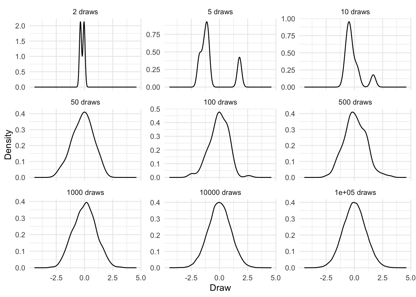
When we use simple linear regression, we assume that our relationship is characterized by the variables and the parameters. If we have two variables, \(Y\) and \(X\), then we could characterize a linear relationship between these as:
\[ Y = \beta_0 + \beta_1 X + \epsilon. \tag{12.1}\]
Here, there are two parameters, also referred to as coefficients: the intercept, \(\beta_0\), and the slope, \(\beta_1\). In Equation 12.1 we are saying that the expected value of \(Y\) is \(\beta_0\) when \(X\) is 0, and that the expected value of \(Y\) will change by \(\beta_1\) units for every one unit change in \(X\). We may then take this relationship to the data that we have to estimate these parameters. The \(\epsilon\) is noise and accounts for deviations away from this relationship. It is this noise that we generally assume to be normally distributed, and it is this that leads to \(Y \sim N(\beta, \sigma^2)\).
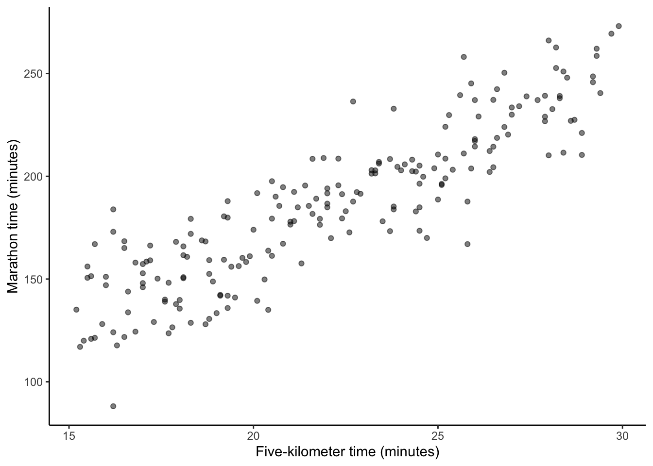
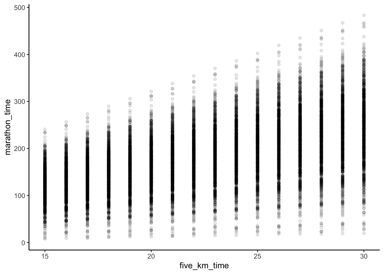
12.2.1 Simulated example: running times
To make this example concrete, we revisit an example from Chapter 9 about the time it takes someone to run five kilometers, compared with the time it takes them to run a marathon (Figure 12.2 (a)). We specified a relationship of 8.4, as that is roughly the ratio between a five-kilometer run and the 42.2-kilometer distance of a marathon. To help the reader, we include the simulation code again here. Notice that it is the noise that is normally distributed, not the variables. We do not require the variables themselves to be normally distributed in order to use linear regression.
set.seed(853)

num_observations <- 200
expected_relationship <- 8.4
fast_time <- 15
good_time <- 30

sim_run_data <-
  tibble(
    five_km_time =
      runif(n = num_observations, min = fast_time, max = good_time),
    noise = rnorm(n = num_observations, mean = 0, sd = 20),
    marathon_time = five_km_time * expected_relationship + noise
  ) |>
  mutate(
    five_km_time = round(x = five_km_time, digits = 1),
    marathon_time = round(x = marathon_time, digits = 1)
  ) |>
  select(-noise)
base_plot <-
sim_run_data |>
ggplot(aes(x = five_km_time, y = marathon_time)) +
geom_point(alpha = 0.5) +
labs(
x = "Five-kilometer time (minutes)",
y = "Marathon time (minutes)"
) +
theme_classic()
# Panel (a)
base_plot
# Panel (b)
base_plot +
geom_smooth(
method = "lm",
se = FALSE,
color = "black",
linetype = "dashed",
formula = "y ~ x"
)
# Panel (c)
base_plot +
geom_smooth(
method = "lm",
se = TRUE,
color = "black",
linetype = "dashed",
formula = "y ~ x"
)
In this simulated example, we know the true values of \(\beta_0\) and \(\beta_1\), which are zero and 8.4, respectively. But our challenge is to see if we can use only the data, and simple linear regression, to recover them. That is, can we use \(x\), which is the five-kilometer time, to produce estimates of \(y\), which is the marathon time, and that we denote by \(\hat{y}\) (by convention, hats are used to indicate that these are, or will be, estimated values) (James et al. [2013] 2021, 61):
\[\hat{y} = \hat{\beta}_0 + \hat{\beta}_1 x.\]
This involves estimating values for \(\beta_0\) and \(\beta_1\). But how should we estimate these coefficients? Even if we impose a linear relationship there are many options because many straight lines could be drawn. But some of those lines would fit the data better than others.
One way we could define a line as being “better” than another, is if it is as close as possible to each of the known \(x\) and \(y\) combinations. There are a lot of candidates for how we define as “close as possible”, but one is to minimize the residual sum of squares. To do this we produce estimates for \(\hat{y}\) based on some guesses of \(\hat{\beta}_0\) and \(\hat{\beta}_1\), given the \(x\). We then work out how wrong, for every observation \(i\), we were (James et al. [2013] 2021, 62):
\[e_i = y_i - \hat{y}_i.\]
To compute the residual sum of squares (RSS), we sum the errors across all the points (taking the square to account for negative differences) (James et al. [2013] 2021, 62):
\[\mbox{RSS} = e^2_1+ e^2_2 +\dots + e^2_n.\]
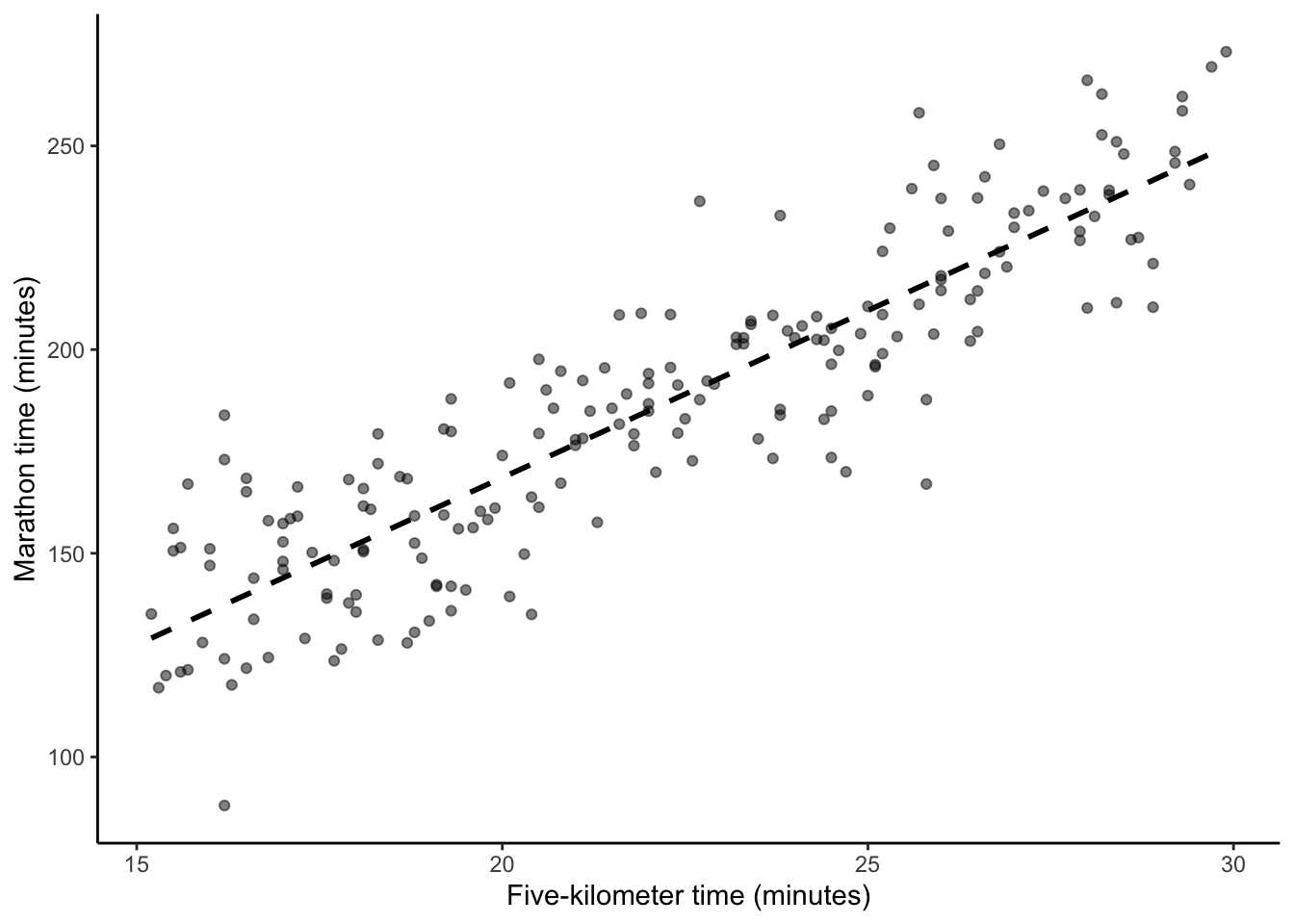
This results in one linear best-fit line (Figure 12.2 (b)), but it is worth reflecting on all the assumptions and decisions that it took to get us to this point.
Underpinning our use of simple linear regression is a belief that there is some “true” relationship between \(X\) and \(Y\). And that this is a linear function of \(X\). We do not, and cannot, know the “true” relationship between \(X\) and \(Y\). All we can do is use our sample to estimate it. But because our understanding depends on that sample, for every possible sample, we would get a slightly different relationship, as measured by the coefficients.
That \(\epsilon\) is a measure of our error—what does the model not know in the small, contained world of the dataset? But it does not tell us whether the model is appropriate outside of the dataset (think, by way of analogy, to the concepts of internal and external validity for experiments introduced in Chapter 8). That requires our judgement and experience.
We can conduct simple linear regression with lm() from base R. We specify the outcome variable first, then ~, followed by the predictor. The outcome variable is the variable of interest, while the predictor is the basis on which we consider that variable. Finally, we specify the dataset.
Before we run a regression, we may want to include a quick check of the class of the variables, and the number of observations, just to ensure that it corresponds with what we were expecting, although we may have done that earlier in the workflow. And after we run it, we may check that our estimate seems reasonable. For instance, (pretending that we had not ourselves imposed this in the simulation) based on our knowledge of the respective distances of a five-kilometer run and a marathon, we would expect \(\beta_1\) to be somewhere between six and ten.
# Check the class and number of observations are as expected
stopifnot(
  class(sim_run_data$marathon_time) == "numeric",
  class(sim_run_data$five_km_time) == "numeric",
  nrow(sim_run_data) == 200
)

sim_run_data_first_model <-
  lm(
    marathon_time ~ five_km_time,
    data = sim_run_data
  )

stopifnot(between(
  sim_run_data_first_model$coefficients[2],
  6,
  10
))
To quickly see the result of the regression, we can use summary().
summary(sim_run_data_first_model)
Call:
lm(formula = marathon_time ~ five_km_time, data = sim_run_data)

Residuals:
    Min      1Q  Median      3Q     Max
-49.289 -11.948   0.153  11.396  46.511

Coefficients:
             Estimate Std. Error t value Pr(>|t|)
(Intercept)    4.4692     6.7517   0.662    0.509
five_km_time   8.2049     0.3005  27.305   <2e-16 ***
---
Signif. codes:  0 '***' 0.001 '**' 0.01 '*' 0.05 '.' 0.1 ' ' 1

Residual standard error: 17.42 on 198 degrees of freedom
Multiple R-squared:  0.7902,    Adjusted R-squared:  0.7891
F-statistic: 745.5 on 1 and 198 DF,  p-value: < 2.2e-16
But we can also use modelsummary() from modelsummary (Table 12.2). The advantage of that approach is that we get a nicely formatted table. We focus initially on those results in the “Five km only” column.
modelsummary(
  list(
    "Five km only" = sim_run_data_first_model,
    "Five km only, centered" = sim_run_data_centered_model
  ),
  fmt = 2
)| Five km only | Five km only, centered | |
|---|---|---|
| (Intercept) | 4.47 | 185.73 |
| (6.75) | (1.23) | |
| five_km_time | 8.20 | |
| (0.30) | ||
| centered_time | 8.20 | |
| (0.30) | ||
| Num.Obs. | 200 | 200 |
| R2 | 0.790 | 0.790 |
| R2 Adj. | 0.789 | 0.789 |
| AIC | 1714.7 | 1714.7 |
| BIC | 1724.6 | 1724.6 |
| Log.Lik. | -854.341 | -854.341 |
| F | 745.549 | 745.549 |
| RMSE | 17.34 | 17.34 |
The top half of Table 12.2 provides our estimated coefficients and standard errors in brackets. And the second half provides some useful diagnostics, which we will not dwell too much in this book. The intercept in the “Five km only” column is the marathon time associated with a hypothetical five-kilometer time of zero minutes. Hopefully this example illustrates the need to always interpret the intercept coefficient carefully. And to disregard it at times. For instance, in this circumstance, we know that the intercept should be zero, and it is just being set to around four because that is the best fit given all the observations were for five-kilometer times between 15 and 30.
The intercept becomes more interpretable when we run the regression using centered five-kilometer time, which we do in the “Five km only, centered” column of Table 12.2. That is, for each of the five-kilometer times we subtract the mean five-kilometer time. In this case, the intercept is interpreted as the expected marathon time for someone who runs five kilometers in the average time. Notice that the slope estimate is unchanged it is only the intercept that has changed.
sim_run_data <-
  sim_run_data |>
  mutate(centered_time = five_km_time - mean(sim_run_data$five_km_time))

sim_run_data_centered_model <-
  lm(
    marathon_time ~ centered_time,
    data = sim_run_data
  )
Following Gelman, Hill, and Vehtari (2020, 84) we recommend considering the coefficients as comparisons, rather than effects. And to use language that makes it clear these are comparisons, on average, based on one dataset. For instance, we may consider that the coefficient on the five-kilometer run time shows how different individuals compare. When comparing the marathon times of individuals in our dataset whose five-kilometer run time differed by one minute, on average we find their marathon times differ by about eight minutes. This makes sense seeing as a marathon is roughly that many times longer than a five-kilometer run.
We can use augment() from broom to add the fitted values and residuals to our original dataset. This allows us to plot the residuals (Figure 12.3).
sim_run_data <-
  augment(
    sim_run_data_first_model,
    data = sim_run_data
  )
# Plot a)
ggplot(sim_run_data, aes(x = .resid)) +
geom_histogram(binwidth = 1) +
theme_classic() +
labs(y = "Number of occurrences", x = "Residuals")
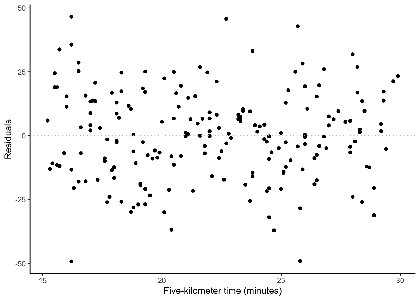
# Plot b)
ggplot(sim_run_data, aes(x = five_km_time, y = .resid)) +
geom_point() +
geom_hline(yintercept = 0, linetype = "dotted", color = "grey") +
theme_classic() +
labs(y = "Residuals", x = "Five-kilometer time (minutes)")
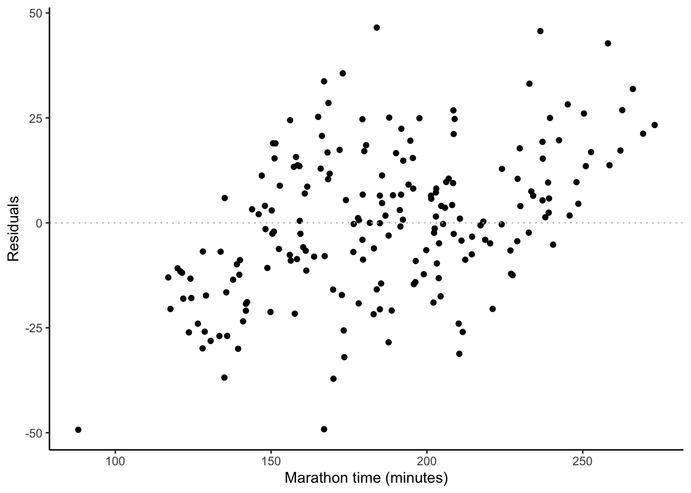
# Plot c)
ggplot(sim_run_data, aes(x = marathon_time, y = .resid)) +
geom_point() +
geom_hline(yintercept = 0, linetype = "dotted", color = "grey") +
theme_classic() +
labs(y = "Residuals", x = "Marathon time (minutes)")
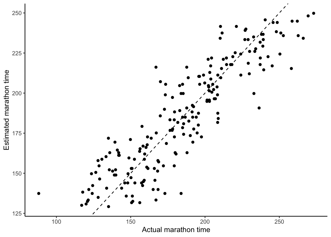
# Plot d)
ggplot(sim_run_data, aes(x = marathon_time, y = .fitted)) +
geom_point() +
geom_abline(intercept = 0, slope = 1, linetype = "dashed") +
theme_classic() +
labs(y = "Estimated marathon time", x = "Actual marathon time")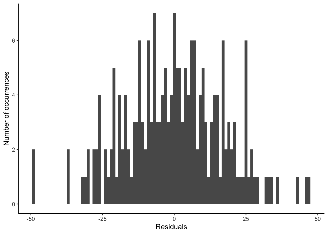
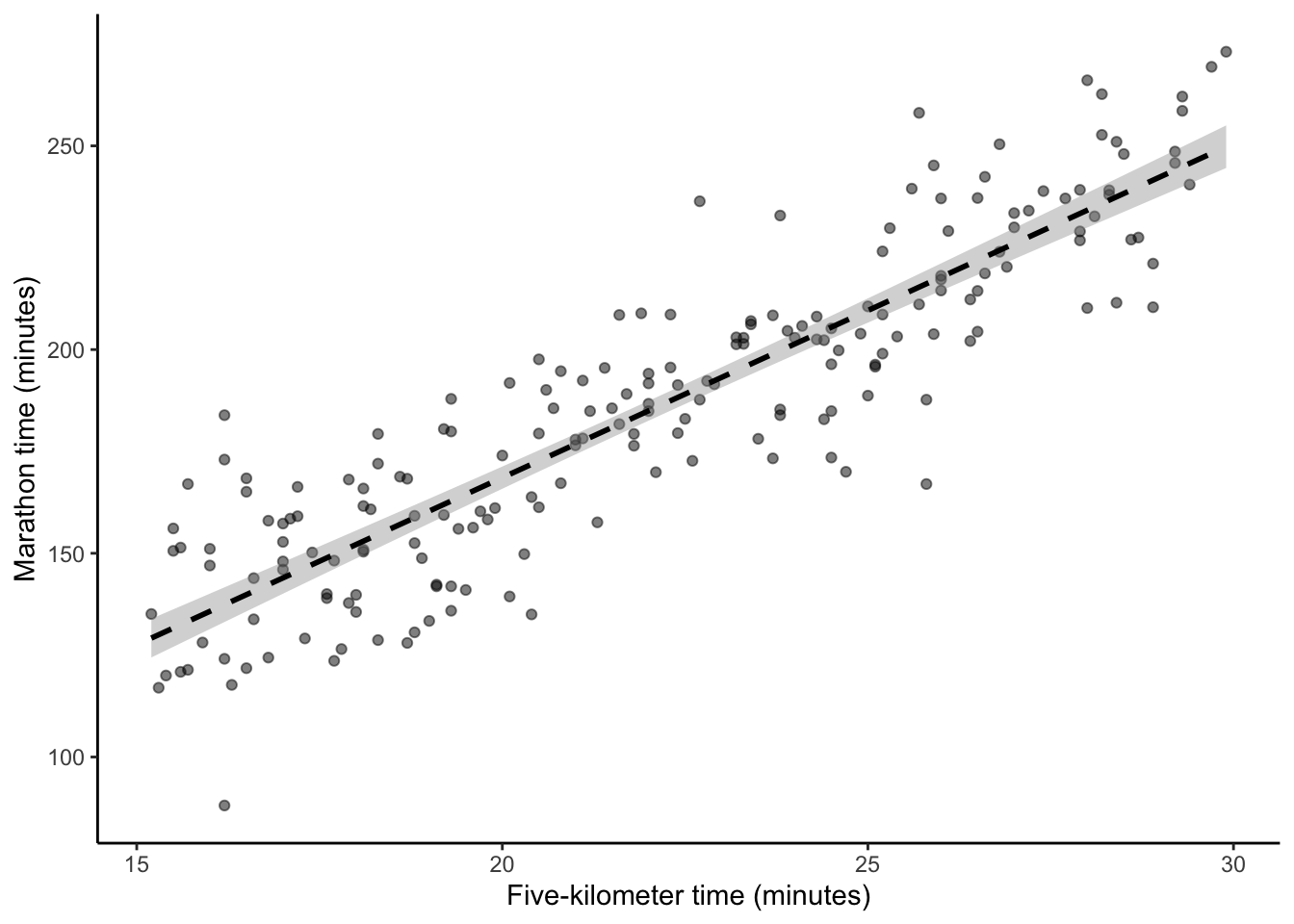
We want to try to speak to the “true” relationship, so we need to try to capture how much we think our understanding depends on the sample that we have to analyze. And this is where the standard error comes in. It guides us, based on many assumptions, about how to think about the estimates of parameters based on the data that we have (Figure 12.2 (c)). Part of this is captured by the fact that standard errors are a function of sample size \(n\), and as the sample size increases, the standard errors decrease.
The most common way to summarize the range of uncertainty for a coefficient is to transform its standard error into a confidence interval. These intervals are often misunderstood to represent a statement of probability about a given realization of the coefficients (i.e. \(\hat\beta\)). In reality, confidence intervals are a statistic whose properties can only be understood “in expectation” (which is equivalent to repeating an experiment many times). A 95 per cent confidence interval is a range, such that there is “approximately a 95 per cent chance that the” range contains the population parameter, which is typically unknown (James et al. [2013] 2021, 66).
When the coefficient follows a Normal distribution, the lower and upper end of a 95 per cent confidence interval range will be about \(\hat{\beta_1} \pm 2 \times \mbox{SE}\left(\hat{\beta_1}\right)\). For instance, in the case of the marathon time example, the lower end is \(8.2 - 2 \times 0.3 = 7.6\) and the upper end is \(8.2 + 2 \times 0.3 = 8.8\), and the true value (which we only know in this case because we simulated it) is 8.4.
We can use this machinery to test claims. For instance, we could claim that there is no relationship between \(X\) and \(Y\), i.e. \(\beta_1 = 0\), as an alternative to a claim that there is some relationship between \(X\) and \(Y\), i.e. \(\beta_1 \neq 0\). This is the null hypothesis testing approach mentioned earlier. In Chapter 8 we needed to decide how much evidence it would take to convince us that our tea taster could distinguish whether milk or tea had been added first. In the same way, here we need to decide if the estimate of \(\beta_1\), which we denote as \(\hat{\beta}_1\), is far enough away from zero for us to be comfortable claiming that \(\beta_1 \neq 0\). If we were very confident in our estimate of \(\beta_1\) then it would not have to be far, but if we were not, then it would have to be substantial. For instance, if the confidence interval contains zero, then we lack evidence to suggest \(\beta_1 \neq 0\). The standard error of \(\hat{\beta}_1\) does an awful lot of work here in accounting for a variety of factors, only some of which it can actually account for, as does our choice as to what it would take to convince us.
We use this standard error and \(\hat{\beta}_1\) to get the “test statistic” or t-statistic:
\[t = \frac{\hat{\beta}_1}{\mbox{SE}(\hat{\beta}_1)}.\]
And we then compare our t-statistic to the t-distribution of Student (1908) to compute the probability of getting this absolute t-statistic or a larger one, if it was the case that \(\beta_1 = 0\). This probability is the p-value. A smaller p-value means there is a smaller “probability of observing something at least as extreme as the observed test statistic” (Gelman, Hill, and Vehtari 2020, 57). Here we use the t-distribution of Student (1908) rather than the Normal distribution, because the t-distribution has slightly larger tails than a standard Normal distribution.
Words! Mere words! How terrible they were! How clear, and vivid, and cruel! One could not escape from them. And yet what a subtle magic there was in them! They seemed to be able to give a plastic form to formless things, and to have a music of their own as sweet as that of viol or of lute. Mere words! Was there anything so real as words?
The Picture of Dorian Gray (Wilde 1891).
We will not make much use of p-values in this book because they are a specific and subtle concept. They are difficult to understand and easy to abuse. Even though they are “little help” for “scientific inference” many disciplines are incorrectly fixated on them (Nelder 1999, 257). One issue is that they embody every assumption of the workflow, including everything that went into gathering and cleaning the data. While p-values have implications if all the assumptions were correct, when we consider the full data science workflow there are usually an awful lot of assumptions. And we do not get guidance from p-values about whether the assumptions are satisfied (Greenland et al. 2016, 339).
A p-value may reject a null hypothesis because the null hypothesis is false, but it may also be that some data were incorrectly gathered or prepared. We can only be sure that the p-value speaks to the hypothesis we are interested in testing if all the other assumptions are correct. There is nothing wrong about using p-values, but it is important to use them in sophisticated and thoughtful ways. Cox (2018) discusses what this requires.
One application where it is easy to see an inappropriate focus on p-values is in power analysis. Power, in a statistical sense, refers to probability of rejecting a null hypothesis that is false. As power relates to hypothesis testing, it also relates to sample size. There is often a worry that a study is “under-powered”, meaning there was not a large enough sample, but rarely a worry that, say, the data were inappropriately cleaned, even though we cannot distinguish between these based only on a p-value. As Meng (2018) and Bradley et al. (2021) demonstrate, a focus on power can blind us from our responsibility to ensure our data are high quality.
Shoulders of giants
Dr Nancy Reid is University Professor in the Department of Statistical Sciences at the University of Toronto. After obtaining a PhD in Statistics from Stanford University in 1979, she took a position as a postdoctoral fellow at Imperial College London. She was appointed as an assistant professor at the University of British Columbia in 1980, and then moved to the University of Toronto in 1986, where she was promoted to full professor in 1988 and served as department chair between 1997 and 2002 (Staicu 2017). Her research focuses on obtaining accurate inference in small-sample regimes and developing inferential procedures for complex models featuring intractable likelihoods. Cox and Reid (1987) examine how re-parameterizing models can simplify inference, Varin, Reid, and Firth (2011) surveys methods for approximating intractable likelihoods, and Reid (2003) overviews inferential procedures in the small-sample regime. Dr Reid was awarded the 1992 COPSS Presidents’ Award, the Royal Statistical Society Guy Medal in Silver in 2016 and in Gold in 2022, and the COPSS Distinguished Achievement Award and Lectureship in 2022.
12.3 Multiple linear regression
To this point we have just considered one explanatory variable. But we will usually have more than one. One approach would be to run separate regressions for each explanatory variable. But compared with separate linear regressions for each, adding more explanatory variables allows for associations between the outcome variable and the predictor variable of interest to be assessed while adjusting for other explanatory variables. The results can be quite different, especially when the explanatory variables are correlated with each other.
We may also like to consider explanatory variables that are not continuous. For instance: pregnant or not; day or night. When there are only two options then we can use a binary variable, which is considered either 0 or 1. If we have a column of character values that only has two values, such as: c("Myles", "Ruth", "Ruth", "Myles", "Myles", "Ruth"), then using this as an explanatory variable in the usual regression set-up would mean that it is treated as a binary variable. If there are more than two levels, then we can use a combination of binary variables, where some baseline outcome gets integrated into the intercept.
12.3.1 Simulated example: running times with rain and humidity
As an example, we add whether it was raining to our simulated relationship between marathon and five-kilometer run times. We then specify that if it was raining, the individual is ten minutes slower than they otherwise would have been.
slow_in_rain <- 10

sim_run_data <-
  sim_run_data |>
  mutate(was_raining = sample(
    c("Yes", "No"),
    size = num_observations,
    replace = TRUE,
    prob = c(0.2, 0.8)
  )) |>
  mutate(
    marathon_time = if_else(
      was_raining == "Yes",
      marathon_time + slow_in_rain,
      marathon_time
    )
  ) |>
  select(five_km_time, marathon_time, was_raining)
We can add additional explanatory variables to lm() with +. Again, we will include a variety of quick tests for class and the number of observations, and add another about missing values. We may not have any idea what the coefficient of rain should be, but if we did not expect it to make them faster, then we could also add a test of that with a wide interval of non-negative values.
stopifnot(
  class(sim_run_data$marathon_time) == "numeric",
  class(sim_run_data$five_km_time) == "numeric",
  class(sim_run_data$was_raining) == "character",
  all(complete.cases(sim_run_data)),
  nrow(sim_run_data) == 200
)

sim_run_data_rain_model <-
  lm(
    marathon_time ~ five_km_time + was_raining,
    data = sim_run_data
  )

stopifnot(
  between(sim_run_data_rain_model$coefficients[3], 0, 20)
  )

summary(sim_run_data_rain_model)
Call:
lm(formula = marathon_time ~ five_km_time + was_raining, data = sim_run_data)

Residuals:
    Min      1Q  Median      3Q     Max
-50.760 -11.942   0.471  11.719  46.916

Coefficients:
               Estimate Std. Error t value Pr(>|t|)
(Intercept)      3.8791     6.8385   0.567 0.571189
five_km_time     8.2164     0.3016  27.239  < 2e-16 ***
was_rainingYes  11.8753     3.2189   3.689 0.000291 ***
---
Signif. codes:  0 '***' 0.001 '**' 0.01 '*' 0.05 '.' 0.1 ' ' 1

Residual standard error: 17.45 on 197 degrees of freedom
Multiple R-squared:  0.791, Adjusted R-squared:  0.7889
F-statistic: 372.8 on 2 and 197 DF,  p-value: < 2.2e-16
The result, in the second column of Table 12.3, shows that when we compare individuals in our dataset who ran in the rain with those who did not, the ones in the rain tended to have a slower time. And this corresponds with what we expect if we look at a plot of the data (Figure 12.4 (a)).
We have included two types of tests here. The ones run before lm() check inputs, and the ones run after lm() check outputs. We may notice that some of the input checks are the same as earlier. One way to avoid having to rewrite tests many times would be to install and load testthat to create a suite of tests of class in say an R file called “class_tests.R”, which are then called using test_file().
For instance, we could save the following as “test_class.R” in a dedicated tests folder.
test_that("Check class", {
  expect_type(sim_run_data$marathon_time, "double")
  expect_type(sim_run_data$five_km_time, "double")
  expect_type(sim_run_data$was_raining, "character")
})
We could save the following as “test_observations.R”
test_that("Check number of observations is correct", {
  expect_equal(nrow(sim_run_data), 200)
})

test_that("Check complete", {
  expect_true(all(complete.cases(sim_run_data)))
})
And finally, we could save the following as “test_coefficient_estimates.R”.
test_that("Check coefficients", {
  expect_gt(sim_run_data_rain_model$coefficients[3], 0)
  expect_lt(sim_run_data_rain_model$coefficients[3], 20)
})
We could then change the regression code to call these test files rather than write them all out.
test_file("tests/test_observations.R")
test_file("tests/test_class.R")

sim_run_data_rain_model <-
  lm(
    marathon_time ~ five_km_time + was_raining,
    data = sim_run_data
  )

test_file("tests/test_coefficient_estimates.R")
It is important to be clear about what we are looking for in the checks of the coefficients. When we simulate data, we put in place reasonable guesses for what the data could look like, and it is similarly reasonable guesses that we test. A failing test is not necessarily a reason to go back and change things, but instead a reminder to look at what is going on in both, and potentially update the test if necessary.
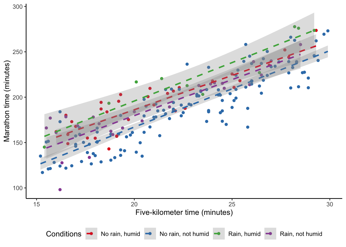
In addition to wanting to include additional explanatory variables, we may think that they are related to each another. For instance, maybe rain really matters if it is also humid that day. We are interested in the humidity and temperature, but also how those two variables interact (Figure 12.4 (b)). We can do this by using * instead of + when we specify the model. When we interact variables in this way, then we almost always need to include the individual variables as well and lm() will do this by default. The result is contained in the third column of Table 12.3.
slow_in_humidity <- 15

sim_run_data <- sim_run_data |>
  mutate(
    humidity = sample(c("High", "Low"), size = num_observations,
                      replace = TRUE, prob = c(0.2, 0.8)),
    marathon_time =
      marathon_time + if_else(humidity == "High", slow_in_humidity, 0),
    weather_conditions = case_when(
      was_raining == "No" & humidity == "Low" ~ "No rain, not humid",
      was_raining == "Yes" & humidity == "Low" ~ "Rain, not humid",
      was_raining == "No" & humidity == "High" ~ "No rain, humid",
      was_raining == "Yes" & humidity == "High" ~ "Rain, humid"
    )
  )
base <-
sim_run_data |>
ggplot(aes(x = five_km_time, y = marathon_time)) +
labs(
x = "Five-kilometer time (minutes)",
y = "Marathon time (minutes)"
) +
theme_classic() +
scale_color_brewer(palette = "Set1") +
theme(legend.position = "bottom")
base +
geom_point(aes(color = was_raining)) +
geom_smooth(
aes(color = was_raining),
method = "lm",
alpha = 0.3,
linetype = "dashed",
formula = "y ~ x"
) +
labs(color = "Was raining")
base +
geom_point(aes(color = weather_conditions)) +
geom_smooth(
aes(color = weather_conditions),
method = "lm",
alpha = 0.3,
linetype = "dashed",
formula = "y ~ x"
) +
labs(color = "Conditions")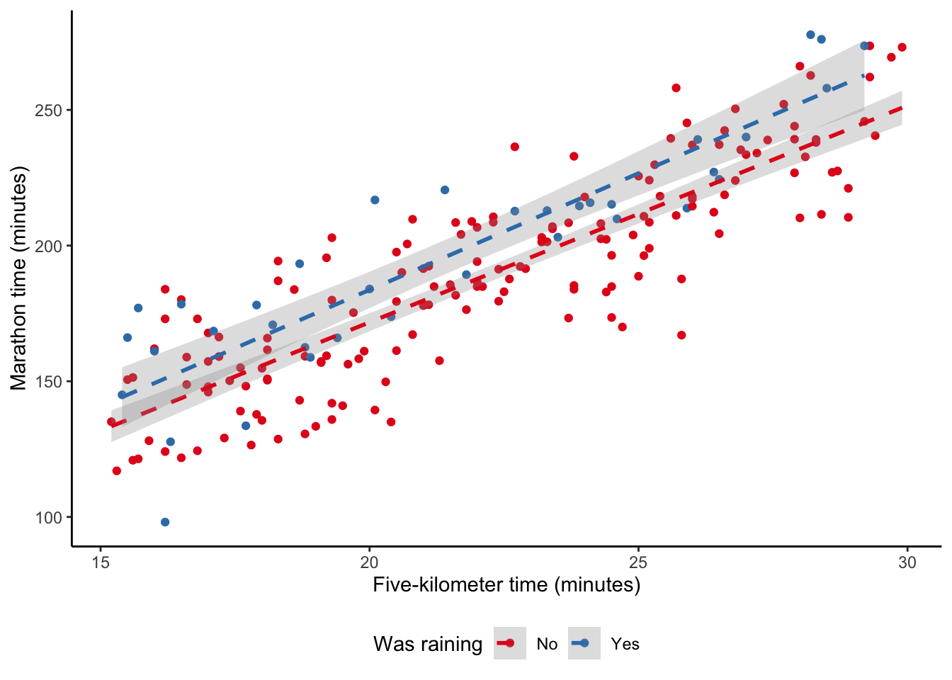
sim_run_data_rain_and_humidity_model <-
  lm(
    marathon_time ~ five_km_time + was_raining * humidity,
    data = sim_run_data
  )

modelsummary(
  list(
    "Five km only" = sim_run_data_first_model,
    "Add rain" = sim_run_data_rain_model,
    "Add humidity" = sim_run_data_rain_and_humidity_model
  ),
  fmt = 2
)| Five km only | Add rain | Add humidity | |
|---|---|---|---|
| (Intercept) | 4.47 | 3.88 | 20.68 |
| (6.75) | (6.84) | (7.12) | |
| five_km_time | 8.20 | 8.22 | 8.24 |
| (0.30) | (0.30) | (0.31) | |
| was_rainingYes | 11.88 | 11.00 | |
| (3.22) | (6.36) | ||
| humidityLow | -18.01 | ||
| (3.45) | |||
| was_rainingYes × humidityLow | 0.92 | ||
| (7.47) | |||
| Num.Obs. | 200 | 200 | 200 |
| R2 | 0.790 | 0.791 | 0.795 |
| R2 Adj. | 0.789 | 0.789 | 0.791 |
| AIC | 1714.7 | 1716.3 | 1719.4 |
| BIC | 1724.6 | 1729.5 | 1739.2 |
| Log.Lik. | -854.341 | -854.169 | -853.721 |
| F | 745.549 | 372.836 | 189.489 |
| RMSE | 17.34 | 17.32 | 17.28 |
There are a variety of threats to the validity of linear regression estimates, and aspects to think about, particularly when using an unfamiliar dataset. We need to address these when we use it, and usually graphs and associated text are sufficient to assuage most of them. Aspects of concern include:
- Linearity of explanatory variables. We are concerned with whether the predictors enter in a linear way. We can usually be convinced there is enough linearity in our explanatory variables for our purposes by using graphs of the variables.
- Homoscedasticity of errors. We are concerned that the errors are not becoming systematically larger or smaller throughout the sample. If that is happening, then we term it heteroscedasticity. Again, graphs of errors, such as Figure 12.3 (b), are used to convince us of this.
- Independence of errors. We are concerned that the errors are not correlated with each other. For instance, if we are interested in weather-related measurement such as average daily temperature, then we may find a pattern because the temperature on one day is likely similar to the temperature on another. We can be convinced that we have satisfied this condition by looking at the residuals compared with observed values, such as Figure 12.3 (c), or estimates compared with actual outcomes, such as Figure 12.3 (d).
- Outliers and other high-impact observations. Finally, we might be worried that our results are being driven by a handful of observations. For instance, thinking back to Chapter 5 and Anscombe’s Quartet, we notice that linear regression estimates would be heavily influenced by the inclusion of one or two particular points. We can become comfortable with this by considering our analysis on various subsets. For instance, randomly removing some observation in the way we did to the US states in Chapter 11.
Those aspects are statistical concerns and relate to whether the model is working. The most important threat to validity and hence the aspect that must be addressed at some length, is whether this model is directly relevant to the research question of interest.
Shoulders of giants
Dr Daniela Witten is the Dorothy Gilford Endowed Chair of Mathematical Statistics and Professor of Statistics & Biostatistics at the University of Washington. After taking a PhD in Statistics from Stanford University in 2010, she joined the University of Washington as an assistant professor. She was promoted to full professor in 2018. One active area of her research is double-dipping which is focused on the effect of sample splitting (Gao, Bien, and Witten 2022). She is an author of the influential Introduction to Statistical Learning (James et al. [2013] 2021). Witten was appointed a Fellow of the American Statistical Association in 2020 and awarded the COPSS Presidents’ Award in 2022.
12.4 Building models
Breiman (2001) describes two cultures of statistical modeling: one focused on inference and the other on prediction. In general, around the time Breiman (2001) was published, various disciplines tended to focus on either inference or prediction. For instance, Jordan (2004) describes how statistics and computer science had been separate for some time, but how the goals of each field were becoming more closely aligned. The rise of data science, and in particular machine learning has meant there is now a need to be comfortable with both (Neufeld and Witten 2021). The two cultures are being brought closer together, and there is an overlap and interaction between prediction and inference. But their separate evolution means there are still considerable cultural differences. As a small example of this, the term “machine learning” tends to be used in computer science, while the term “statistical learning” tends to be used in statistics, even though they usually refer to the same machinery.
In this book we will focus on inference using the probabilistic programming language Stan to fit models in a Bayesian framework, and interface with it using rstanarm. Inference and forecasting have different cultures, ecosystems, and priorities. You should try to develop a comfort in both. One way these different cultures manifest is in language choice. The primary language in this book is R, and for the sake of consistency we focus on that here. But there is an extensive culture, especially but not exclusively focused on prediction, that uses Python. We recommend focusing on only one language and approach initially, but after developing that initial familiarity it is important to become multilingual. We introduce prediction based on Python in Online Appendix 14.
We will again not go into the details, but running a regression in a Bayesian setting is similar to the frequentist approach that underpins lm(). The main difference from a regression point of view, is that the parameters involved in the models (i.e. \(\beta_0\), \(\beta_1\), etc) are considered random variables, and so themselves have associated probability distributions. In contrast, the frequentist paradigm assumes that any randomness from these coefficients comes from a parametric assumption on the distribution of the error term, \(\epsilon\).
Before we run a regression in a Bayesian framework, we need to decide on a starting probability distribution for each of these parameters, which we call a “prior”. While the presence of priors adds some additional complication, it has several advantages, and we will discuss the issue of priors in more detail below. This is another reason for the workflow advocated in this book: the simulation stage leads directly to priors. We will again specify the model that we are interested in, but this time we include priors.
\[ \begin{aligned} y_i|\mu_i, \sigma &\sim \mbox{Normal}(\mu_i, \sigma) \\ \mu_i &= \beta_0 +\beta_1x_i\\ \beta_0 &\sim \mbox{Normal}(0, 2.5) \\ \beta_1 &\sim \mbox{Normal}(0, 2.5) \\ \sigma &\sim \mbox{Exponential}(1) \\ \end{aligned} \]
We combine information from the data with the priors to obtain posterior distributions for our parameters. Inference is then carried out based on analyzing posterior distributions.
Another aspect that is different between Bayesian approaches and the way we have been doing modeling to this point, is that Bayesian models will usually take longer to run. Because of this, it can be useful to run the model in a separate R script and then save it with saveRDS(). With sensible Quarto chunk options for “eval” and “echo” (see Chapter 3), the model can then be read into the Quarto document with readRDS() rather than being run every time the paper is compiled. In this way, the model delay is only imposed once for a given model. It can also be useful to add beep() from beepr to the end of the model, to get an audio notification when the model is done.
sim_run_data_first_model_rstanarm <-
  stan_glm(
    formula = marathon_time ~ five_km_time + was_raining,
    data = sim_run_data,
    family = gaussian(),
    prior = normal(location = 0, scale = 2.5),
    prior_intercept = normal(location = 0, scale = 2.5),
    prior_aux = exponential(rate = 1),
    seed = 853
  )

beep()

saveRDS(
  sim_run_data_first_model_rstanarm,
  file = "sim_run_data_first_model_rstanarm.rds"
)
sim_run_data_first_model_rstanarm <-
readRDS(file = "sim_run_data_first_model_rstanarm.rds")We use stan_glm() with the “gaussian()” family to specify multiple linear regression and the model formula is written in the same way as base R and `rstanarm``. We have explicitly added the default priors, as we see this as good practice, although strictly this is not necessary.
The estimation results, which are in the first column of Table 12.4, are not quite what we expect. For instance, the rate of increase in marathon times is estimated to be around three minutes per minute of increase in five-kilometer time, which seems low given the ratio of a five-kilometer run to marathon distance.
12.4.1 Picking priors
The issue of picking priors is a challenging one and the subject of extensive research. For the purposes of this book, using the rstanarm defaults is fine. But even if they are just the default, priors should be explicitly specified in the model and included in the function. This is to make it clear to others what has been done. We could use default_prior_intercept() and default_prior_coef() to find the default priors in rstanarm and then explicitly include them in the model.
It is normal to find it difficult to know what prior to specify. Getting started by adapting someone else’s rstanarm code is perfectly fine. If they have not specified their priors, then we can use the helper function prior_summary(), to find out which priors were used.
prior_summary(sim_run_data_first_model_rstanarm)Priors for model 'sim_run_data_first_model_rstanarm'
------
Intercept (after predictors centered)
~ normal(location = 0, scale = 2.5)
Coefficients
~ normal(location = [0,0], scale = [2.5,2.5])
Auxiliary (sigma)
~ exponential(rate = 1)
------
See help('prior_summary.stanreg') for more detailsWe are interested in understanding what the priors imply before we involve any data. We do this by implementing prior predictive checks. This means simulating from the priors to look at what the model implies about the possible magnitude and direction of the relationships between the explanatory and outcome variables. This process is no different to all the other simulation that we have done to this point.
draws <- 1000

priors <-
  tibble(
    sigma = rep(rexp(n = draws, rate = 1), times = 16),
    beta_0 = rep(rnorm(n = draws, mean = 0, sd = 2.5), times = 16),
    beta_1 = rep(rnorm(n = draws, mean = 0, sd = 2.5), times = 16),
    five_km_time = rep(15:30, each = draws),
    mu = beta_0 + beta_1 * five_km_time
  ) |>
  rowwise() |>
  mutate(
    marathon_time = rnorm(n = 1, mean = mu, sd = sigma)
  )
priors |>
ggplot(aes(x = marathon_time)) +
geom_histogram(binwidth = 10) +
theme_classic()
priors |>
ggplot(aes(x = five_km_time, y = marathon_time)) +
geom_point(alpha = 0.1) +
theme_classic()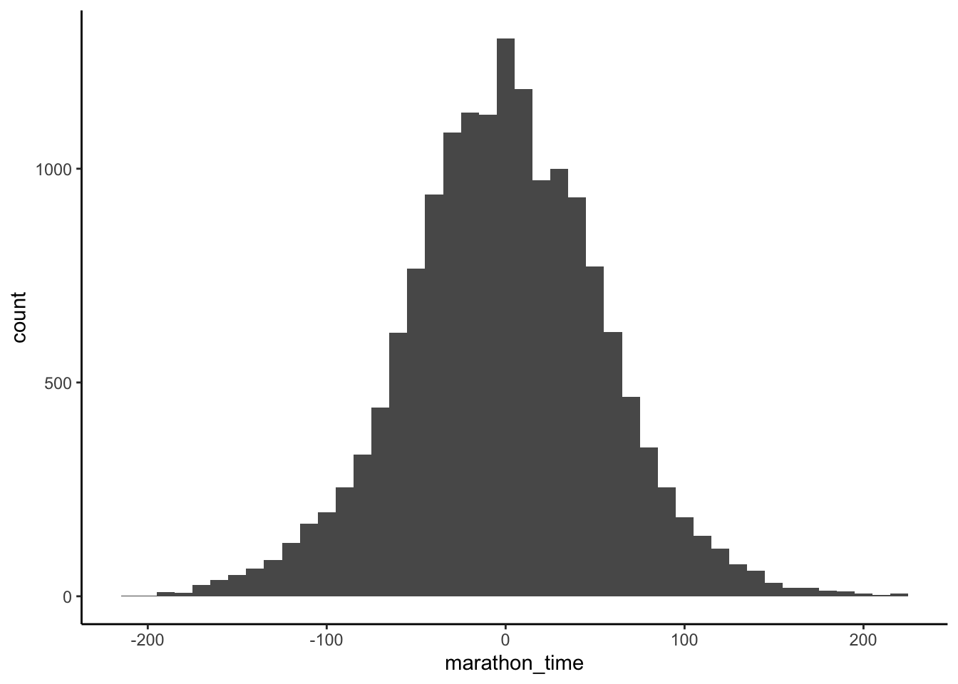
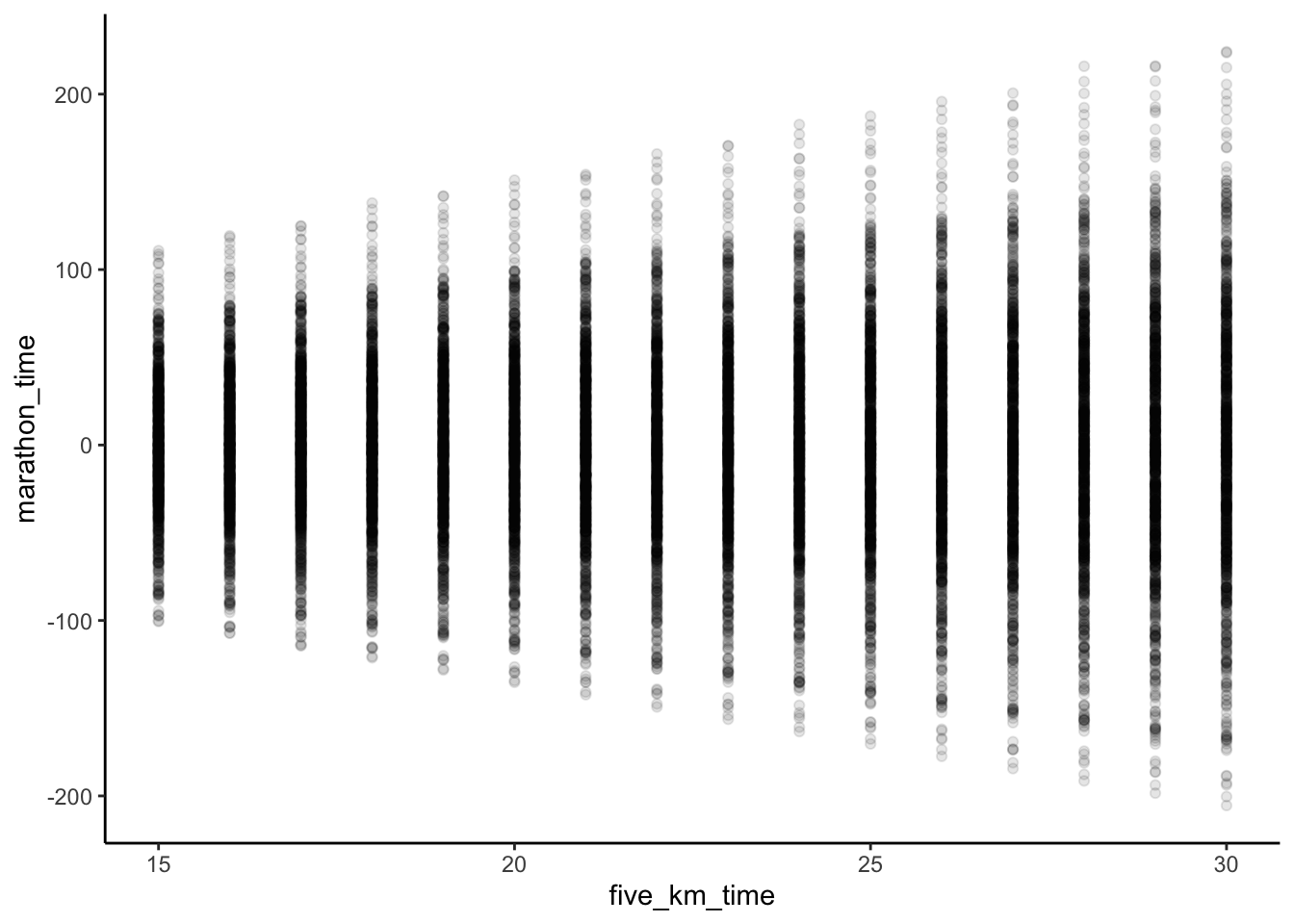
Figure 12.5 suggests our model has been poorly constructed. Not only are there world record marathon times, but there are also negative marathon times! One issue is that our prior for \(\beta_1\) does not take in all the information that we know. We know that a marathon is about eight times longer than a five-kilometer run and so we could center the prior for \(\beta_1\) around that. Our re-specified model is:
\[ \begin{aligned} y_i|\mu_i, \sigma &\sim \mbox{Normal}(\mu_i, \sigma) \\ \mu_i &= \beta_0 +\beta_1x_i\\ \beta_0 &\sim \mbox{Normal}(0, 2.5) \\ \beta_1 &\sim \mbox{Normal}(8, 2.5) \\ \sigma &\sim \mbox{Exponential}(1) \\ \end{aligned} \] And we can see from prior prediction checks that it seems more reasonable (Figure 12.6).
draws <- 1000

updated_priors <-
  tibble(
    sigma = rep(rexp(n = draws, rate = 1), times = 16),
    beta_0 = rep(rnorm(n = draws, mean = 0, sd = 2.5), times = 16),
    beta_1 = rep(rnorm(n = draws, mean = 8, sd = 2.5), times = 16),
    five_km_time = rep(15:30, each = draws),
    mu = beta_0 + beta_1 * five_km_time
  ) |>
  rowwise() |>
  mutate(
    marathon_time = rnorm(n = 1, mean = mu, sd = sigma)
  )
updated_priors |>
ggplot(aes(x = marathon_time)) +
geom_histogram(binwidth = 10) +
theme_classic()
updated_priors |>
ggplot(aes(x = five_km_time, y = marathon_time)) +
geom_point(alpha = 0.1) +
theme_classic()
If we were not sure what to do then rstanarm could help to improve the specified priors, by scaling them based on the data. Specify the prior that you think is reasonable, even if this is just the default, and include it in the function, but also include “autoscale = TRUE”, and rstanarm will adjust the scale. When we re-run our model with these updated priors and allowing auto-scaling we get much better results, which are in the second column of Table 12.4. You can then add those to the written-out model instead.
sim_run_data_second_model_rstanarm <-
  stan_glm(
    formula = marathon_time ~ five_km_time + was_raining,
    data = sim_run_data,
    family = gaussian(),
    prior = normal(location = 8, scale = 2.5, autoscale = TRUE),
    prior_intercept = normal(0, 2.5, autoscale = TRUE),
    prior_aux = exponential(rate = 1, autoscale = TRUE),
    seed = 853
  )

saveRDS(
  sim_run_data_second_model_rstanarm,
  file = "sim_run_data_second_model_rstanarm.rds"
)modelsummary(
list(
"Non-scaled priors" = sim_run_data_first_model_rstanarm,
"Auto-scaling priors" = sim_run_data_second_model_rstanarm
),
fmt = 2
)| Non-scaled priors | Auto-scaling priors | |
|---|---|---|
| (Intercept) | -67.50 | 8.66 |
| five_km_time | 3.47 | 7.90 |
| was_rainingYes | 0.12 | 9.23 |
| Num.Obs. | 100 | 100 |
| R2 | 0.015 | 0.797 |
| R2 Adj. | -1.000 | 0.790 |
| Log.Lik. | -678.336 | -425.193 |
| ELPD | -679.5 | -429.0 |
| ELPD s.e. | 3.3 | 8.9 |
| LOOIC | 1359.0 | 858.0 |
| LOOIC s.e. | 6.6 | 17.8 |
| WAIC | 1359.0 | 857.9 |
| RMSE | 175.52 | 16.85 |
As we used the “autoscale = TRUE” option, it can be helpful to look at how the priors were updated with prior_summary() from rstanarm.
prior_summary(sim_run_data_second_model_rstanarm)Priors for model 'sim_run_data_second_model_rstanarm'
------
Intercept (after predictors centered)
Specified prior:
~ normal(location = 0, scale = 2.5)
Adjusted prior:
~ normal(location = 0, scale = 95)
Coefficients
Specified prior:
~ normal(location = [8,8], scale = [2.5,2.5])
Adjusted prior:
~ normal(location = [8,8], scale = [ 22.64,245.52])
Auxiliary (sigma)
Specified prior:
~ exponential(rate = 1)
Adjusted prior:
~ exponential(rate = 0.026)
------
See help('prior_summary.stanreg') for more details12.4.2 Posterior distribution
Having built a Bayesian model, we may want to look at what it implies (Figure 12.7). One way to do this is to consider the posterior distribution.
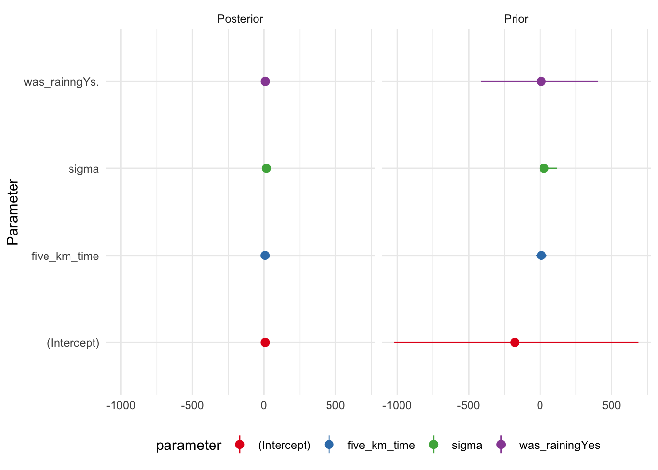
One way to use the posterior distribution is to consider whether the model is doing a good job of fitting the data. The idea is that if the model is doing a good job of fitting the data, then the posterior should be able to be used to simulate data that are like the actual data (Gelman et al. 2020). We can implement a posterior predictive check with pp_check() from rstanarm (Figure 12.7 (a)). This compares the actual outcome variable with simulations from the posterior distribution. And we can compare the posterior with the prior with posterior_vs_prior() to see how much the estimates change once data are taken into account (Figure 12.7 (b)). Helpfully, pp_check() and posterior_vs_prior() return ggplot2 objects so we can modify the look of them in the normal way we manipulate graphs. These checks and discussion would typically just be briefly mentioned in the main content of a paper, with the detail and graphs added to a dedicated appendix.
pp_check(sim_run_data_second_model_rstanarm) +
  theme_classic() +
  theme(legend.position = "bottom")

posterior_vs_prior(sim_run_data_second_model_rstanarm) +
  theme_minimal() +
  scale_color_brewer(palette = "Set1") +
  theme(legend.position = "bottom") +
  coord_flip()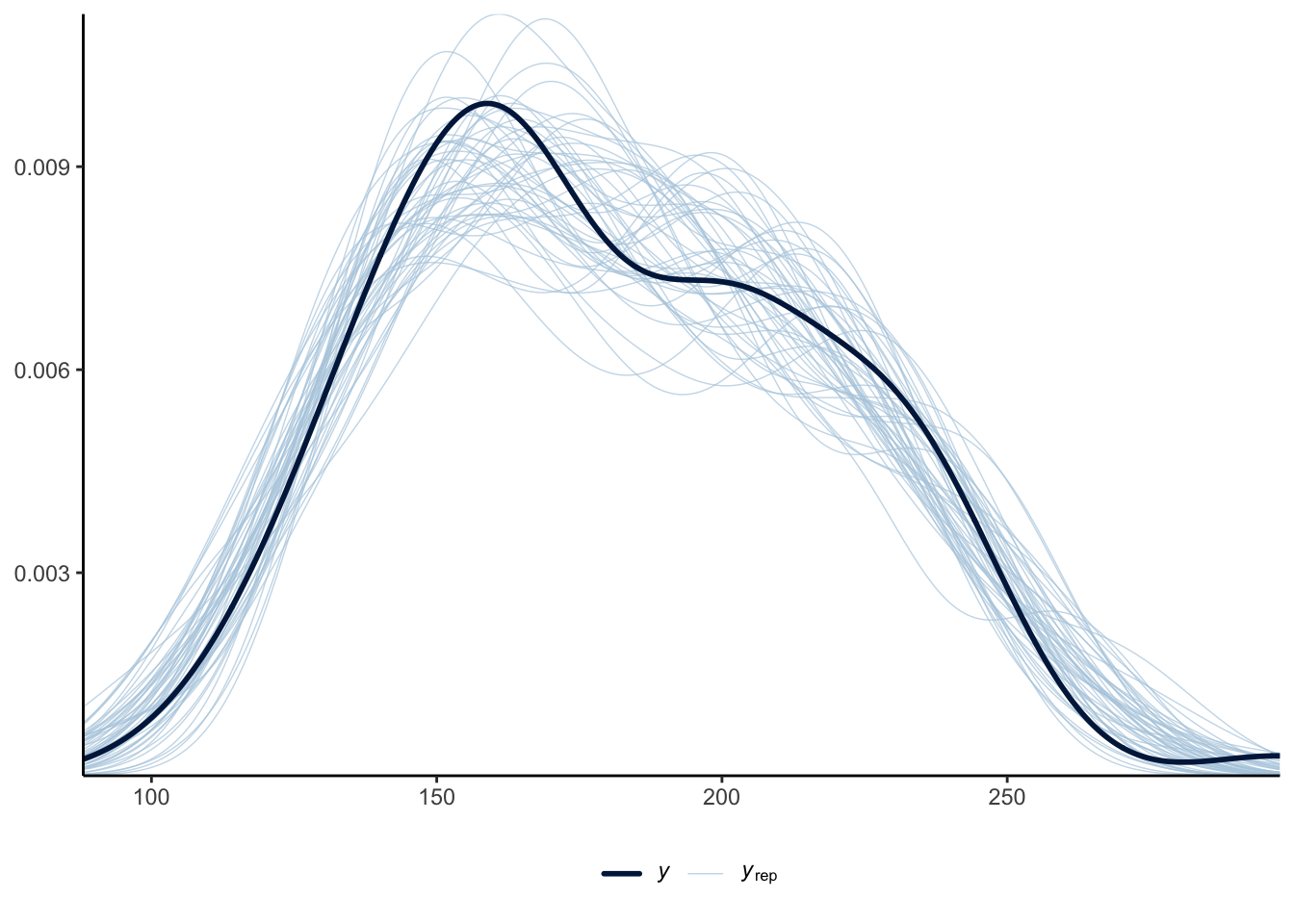
With a simple model like this, the differences between the prediction and inference approaches are minimal. But as model or data complexity increases these differences can become important.
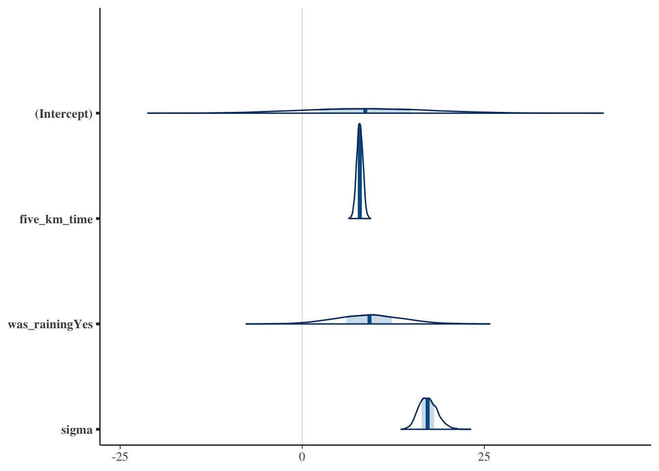
We have already discussed confidence intervals and the Bayesian equivalent to a confidence interval is called a “credibility interval”, and reflects two points where there is a certain probability mass between them, in this case 95 per cent. Bayesian estimation provides a distribution for each coefficient. This means there is an infinite number of points that we could use to generate this interval. The entire distribution should be shown graphically (Figure 12.8). This might be using a cross-referenced appendix.
plot(
  sim_run_data_second_model_rstanarm,
  "areas"
)
12.4.3 Diagnostics
The final aspect that we would like to check is a practical matter. rstanarm uses a sampling algorithm called Markov chain Monte Carlo (MCMC) to obtain samples from the posterior distributions of interest. We need to quickly check for the existence of signs that the algorithm ran into issues. We consider a trace plot, such as Figure 12.9 (a), and a Rhat plot, such as Figure 12.9 (b). These would typically go in a cross-referenced appendix.
plot(sim_run_data_second_model_rstanarm, "trace")

plot(sim_run_data_second_model_rstanarm, "rhat")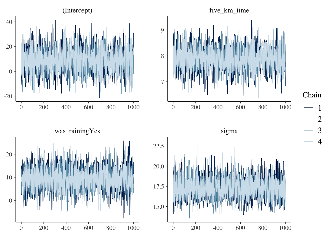
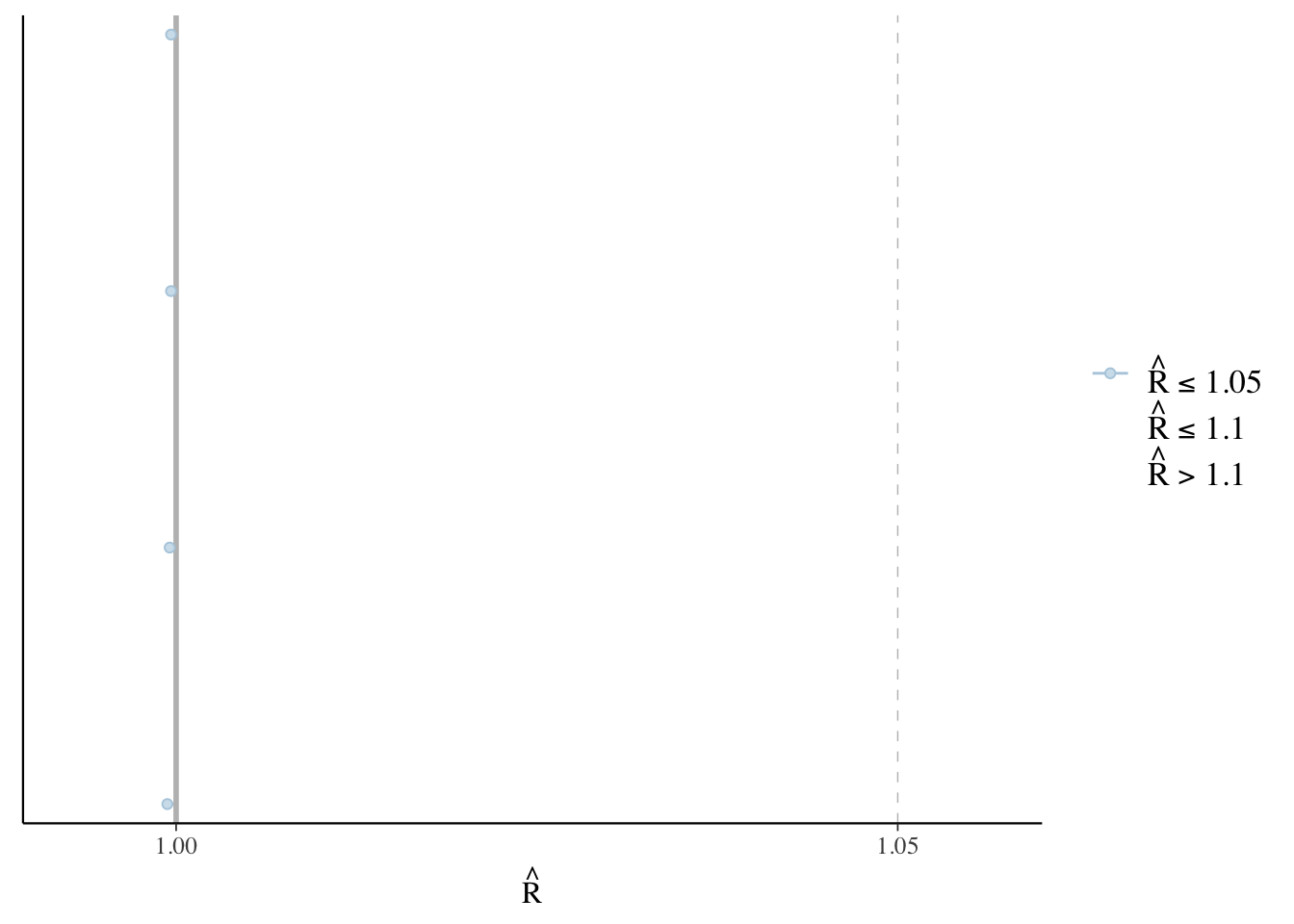
In the trace plot, we are looking for lines that appear to bounce around, but are horizontal, and have a nice overlap between the chains. The trace plot in Figure 12.9 (a) does not suggest anything out of the ordinary. Similarly, with the Rhat plot, we are looking for everything to be close to 1, and ideally no more than 1.1. Again Figure 12.9 (b) is an example that does not suggest any problems. If these diagnostics are not like this, then simplify the model by removing or modifying predictors, change the priors, and re-run it.
12.4.4 Parallel processing
Sometimes code is slow because the computer needs to do the same thing many times. We may be able to take advantage of this and enable these jobs to be done at the same time using parallel processing. This is especially the case when estimating Bayesian models.
After installing and loading tictoc we can use tic() and toc() to time various aspects of our code. This is useful with parallel processing, but also more generally, to help us find out where the largest delays are.
tic("First bit of code")
print("Fast code")
[1] "Fast code"toc()First bit of code: 0 sec elapsedtic("Second bit of code")
Sys.sleep(3)
print("Slow code")[1] "Slow code"toc()Second bit of code: 3.008 sec elapsedAnd so we know that there is something slowing down the code. (In this artificial case it is Sys.sleep() causing a delay of three seconds.)
We could use parallel which is part of base R to run functions in parallel. We could also use future which brings additional features. After installing and loading future we use plan() to specify whether we want to run things sequentially (“sequential”) or in parallel (“multisession”). We then wrap what we want this applied to within future().
To see this in action we will create a dataset and then implement a function on a row-wise basis.
simulated_data <-
  tibble(
    random_draws = runif(n = 1000000, min = 0, max = 1000) |> round(),
    more_random_draws = runif(n = 1000000, min = 0, max = 1000) |> round()
  )

plan(sequential)

tic()
simulated_data <-
  simulated_data |>
  rowwise() |>
  mutate(which_is_smaller =
           min(c(random_draws,
                 more_random_draws)))
toc()

plan(multisession)

tic()
simulated_data <-
  future(simulated_data |>
           rowwise() |>
           mutate(which_is_smaller =
                    min(c(
                      random_draws,
                      more_random_draws
                    ))))
toc()
The sequential approach takes about 5 seconds, while the multisession approach takes about 0.3 seconds.
In the case of estimating Bayesian models many packages such as rstanarm have support for parallel processing built in through cores.
12.5 Concluding remarks
In this chapter we have considered linear models. We established a foundation for analysis, and described some essential approaches. We have also skimmed over a lot. This chapter and the next should be considered together. These provide you with enough to get started, but for doing more than that, going through the modeling books recommended in Chapter 18.
12.6 Exercises
Practice
- (Plan) Consider the following scenario: A person is interested in the heights of all the buildings in London. They walk around the city counting the number of floors for each building, and noting the year of construction. Please sketch what that dataset could look like and then sketch a graph that you could build to show all observations.
- (Simulate) Please further consider the scenario described and simulate the situation, along with three predictors that are associated the count of the number of levels. Please include at least ten tests based on the simulated data. Submit a link to a GitHub Gist that contains your code.
- (Acquire) Please describe one possible source of such a dataset.
- (Explore) Please use
ggplot2to build the graph that you sketched. Then userstanarmto build a model with number of floors as an outcome and the year of construction as a predictor. Submit a link to a GitHub Gist that contains your code. - (Communicate) Please write two paragraphs about what you did.
Quiz
- Please simulate the situation in which there are two predictors, “race” and “gender”, and one outcome variable, “vote_preference”, which is imperfectly related to them. Submit a link to a GitHub Gist that contains your code.
- Please write a linear relationship between some outcome variable, Y, and some predictor, X. What is the intercept term? What is the slope term? What would adding a hat to these indicate?
- Which of the following are examples of linear models (select all that apply)?
lm(y ~ x_1 + x_2 + x_3, data = my_data)lm(y ~ x_1 + x_2^2 + x_3, data = my_data)lm(y ~ x_1 * x_2 + x_3, data = my_data)lm(y ~ x_1 + x_1^2 + x_2 + x_3, data = my_data)
- What is the least squares criterion? Similarly, what is RSS and what are we trying to do when we run least squares regression?
- What is bias (in a statistical context)?
- Consider five variables: earth, fire, wind, water, and heart. Please simulate a scenario where heart depends on the other four, which are independent of each other. Then please write R code that would fit a linear regression model to explain heart as a function of the other variables. Submit a link to a GitHub Gist that contains your code.
- According to Greenland et al. (2016), p-values test (pick one):
- All the assumptions about how the data were generated (the entire model), not just the targeted hypothesis it is supposed to test (such as a null hypothesis).
- Whether the hypothesis targeted for testing is true or not.
- A dichotomy whereby results can be declared “statistically significant”.
- According to Greenland et al. (2016), a p-value may be small because (select all that apply):
- The targeted hypothesis is false.
- The study protocols were violated.
- It was selected for presentation based on its small size.
- Please explain what a p-value is, using only the term itself (i.e. “p-value”) and words that are amongst the 1,000 most common in the English language according to the XKCD Simple Writer. (Please write one or two paragraphs.)
- What is power (in a statistical context)?
- Look at the list of people awarded the COPSS Presidents’ Award or the Guy Medal in Gold and write a short biography of them in the style of the “Shoulders of giants” entries in this book.
- Discuss, with the help of examples and citations, the quote from McElreath ([2015] 2020, 162) included toward the start of this chapter. Write at least three paragraphs.
Class activities
- Use the starter folder and create a new repo.
- We are interested in understanding the relationship between bill length and depth for Adelie penguins using
palmerpenguins. Begin by sketching and simulating. - Then add three graphs to the data section: one of each variable separately and a third of the relationship between the two.
- Then in the model section, write out the model. Use
rstanarmto estimate a linear model between the two variables in an R script. - Read that model into the results section and use
modelsummaryto create a summary table.
- We are interested in understanding the relationship between bill length and depth for Adelie penguins using
palmerpenguins::penguins |>
  filter(species == "Adelie") |>
  ggplot(aes(x = bill_length_mm, y = bill_depth_mm)) +
  geom_point()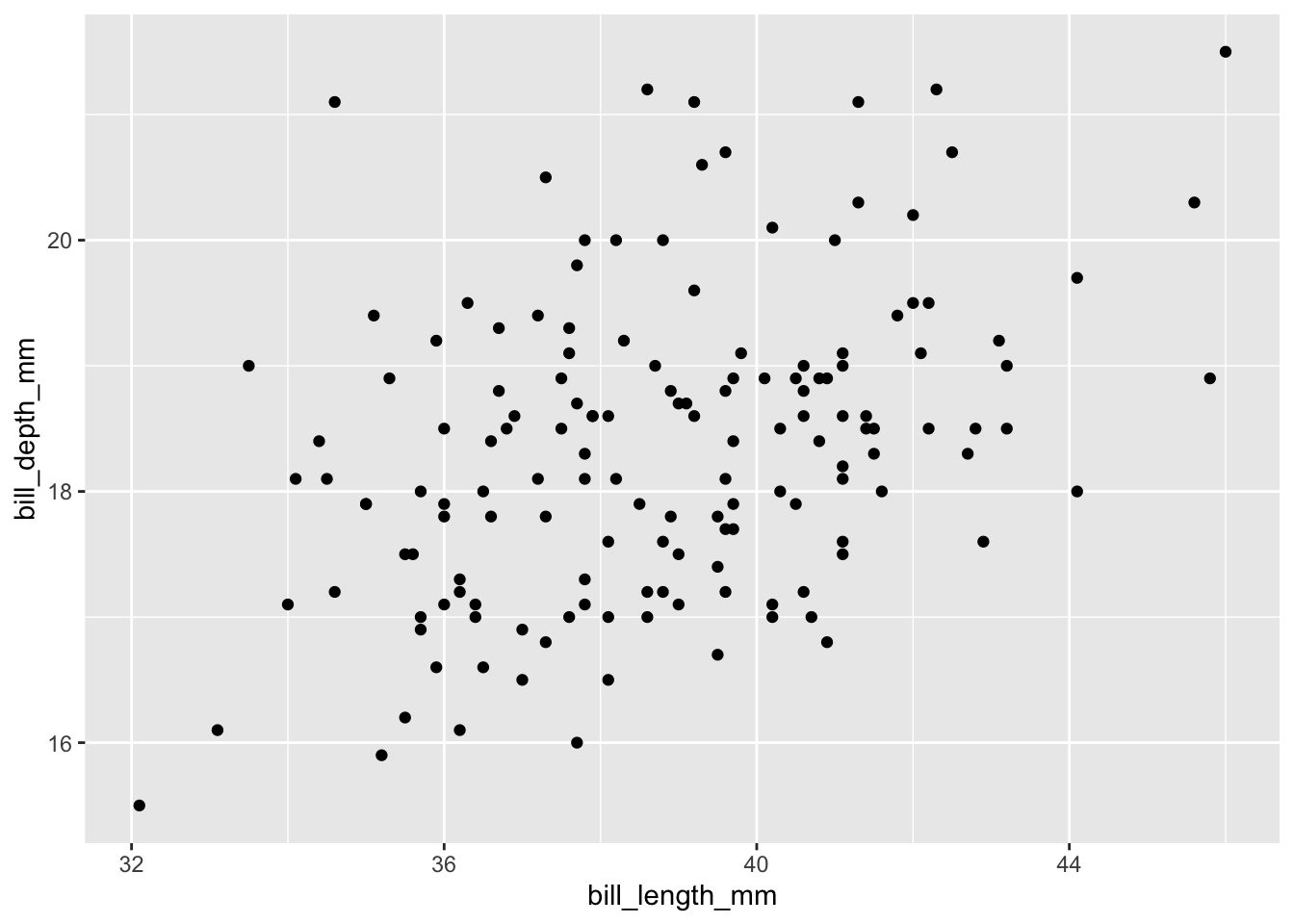
- (This question is based on Gelman and Vehtari (2024, 32).) Please follow the instructions here to make a paper plane. Measure:
- the width of the wings;
- the length of the wings;
- the height of the winglets;
- in a safe space, fly your plane and measure for how long it stays in the air.
Combine your data with those of the rest of the class in a table that looks like Table 12.5. Then use linear regression to explore the relationship between the dependent and independent variables. Based on the results, how would you change your plane design if you were to do this exercise again?
| Wing width (mm) | Wing length (mm) | Winglet height (mm) | Flying time (sec) |
|---|---|---|---|
| ... | ... | ... | ... |
- Imagine that we add FIPS code as an explanatory variable in a linear regression model explaining inflation, by US county. Please discuss the likely effect of this and whether it is a good idea. You may want to simulate the situation to help you think it through more clearly.
- Imagine that we add latitude and longitude as explanatory variables in a regression trying to explain flu prevalence in each UK city and town. Please discuss the likely effect of this and whether it is a good idea. You may want to simulate the situation to help you think it through more clearly.
- In Shakespeare’s Julius Caesar, the character Cassius famously says:
The fault, dear Brutus, is not in our stars,
But in ourselves, that we are underlings.
Please discuss p-values, the common, but potentially misleading, use of significance stars in regression tables, and Ioannidis (2005), with reference to this quote. - Imagine that a variance estimate ends up negative. Please discuss.
Task
Allow that the true data generating process is a Normal distribution with mean of one, and standard deviation of 1. We obtain a sample of 1,000 observations using some instrument. Simulate the following situation:
- Unknown to us, the instrument has a mistake in it, which means that it has a maximum memory of 900 observations, and begins over-writing at that point, so the final 100 observations are actually a repeat of the first 100.
- We employ a research assistant to clean and prepare the dataset. During the process of doing this, unknown to us, they accidentally change half of the negative draws to be positive.
- They additionally, accidentally, change the decimal place on any value between 1 and 1.1, so that, for instance 1 becomes 0.1, and 1.1 would become 0.11.
- You finally get the cleaned dataset and are interested in understanding whether the mean of the true data generating process is greater than 0.
Write at least two pages about what you did and what you found. Also discuss what effect the issues had, and what steps you can put in place to ensure actual analysis has a chance to flag some of these issues.
Use Quarto, and include an appropriate title, author, date, link to a GitHub repo, and citations to produce a draft. Following this, please pair with another student and exchange your written work. Update it based on their feedback, and be sure to acknowledge them by name in your paper. Submit a PDF.
Given the small sample size in the example of 20, we strictly should use the finite-sample adjustment, but as this is not the focus of this book we will move forward with the general approach.↩︎