SELECT
    surname
FROM
politicians;Online Appendix H — SQL essentials
Prerequisites
- Read Early History of SQL, (Chamberlin 2012)
- An interesting overview of the development of SQL.
Key concepts and skills
- While we could use various R package, or write SQL within RStudio, the industry demand for SQL, makes it worthwhile learning independently of R, at least initially.
- SQLite is one flavor of SQL, and we can use DB Browser for SQLite as an IDE for SQL.
Key packages and functions
BETWEENDESCDISTINCTFROMGROUP BYLEFT JOINLIKELIMITORORDER BYSELECTUPDATEWHERE
H.1 Introduction
Structured Query Language (SQL) (“see-quell” or “S.Q.L.”) is used with relational databases. A relational database is a collection of at least one table, and a table is just some data organized into rows and columns. If there is more than one table in the database, then there should be some column that links them. An example is the AustralianPoliticians datasets that are used in Appendix A. Using SQL feels a bit like HTML/CSS in terms of being halfway between markup and programming. One fun aspect is that, by convention, commands are written in upper case. Another is that line spaces mean nothing: include them or do not, but always end a SQL command in a semicolon;
SQL was developed in the 1970s at IBM. SQL is an especially popular way of working with data. There are many “flavors” of SQL, including both closed and open options. Here we introduce SQLite, which is open source, and pre-installed on Macs. Windows users can install it from here.
Advanced SQL users do a lot with it alone, but even just having a working knowledge of SQL increases the number of datasets that we can access. A working knowledge of SQL is especially useful for our efficiency because a large number of datasets are stored on SQL servers, and being able to get data from them ourselves is handy.
We could use SQL within RStudio, especially drawing on DBI (R Special Interest Group on Databases (R-SIG-DB), Wickham, and Müller 2022). Although given the demand for SQL skills, independent of demand for R skills, it may be a better idea, from a career perspective to have a working knowledge of it that is independent of RStudio. We can consider many SQL commands as straightforward variants of the dplyr verbs that we have used throughout this book. Indeed, if we wanted to stay within R, then dbplyr (Wickham, Girlich, and Ruiz 2022) would explicitly allow us to use dplyr functions and would then automatically translate them into SQL. Having used mutate(), filter(), and left_join() in the tidyverse means that many of the core SQL commands will be familiar. That means that the main difficulty will be getting on top of the order of operations because SQL can be pedantic.
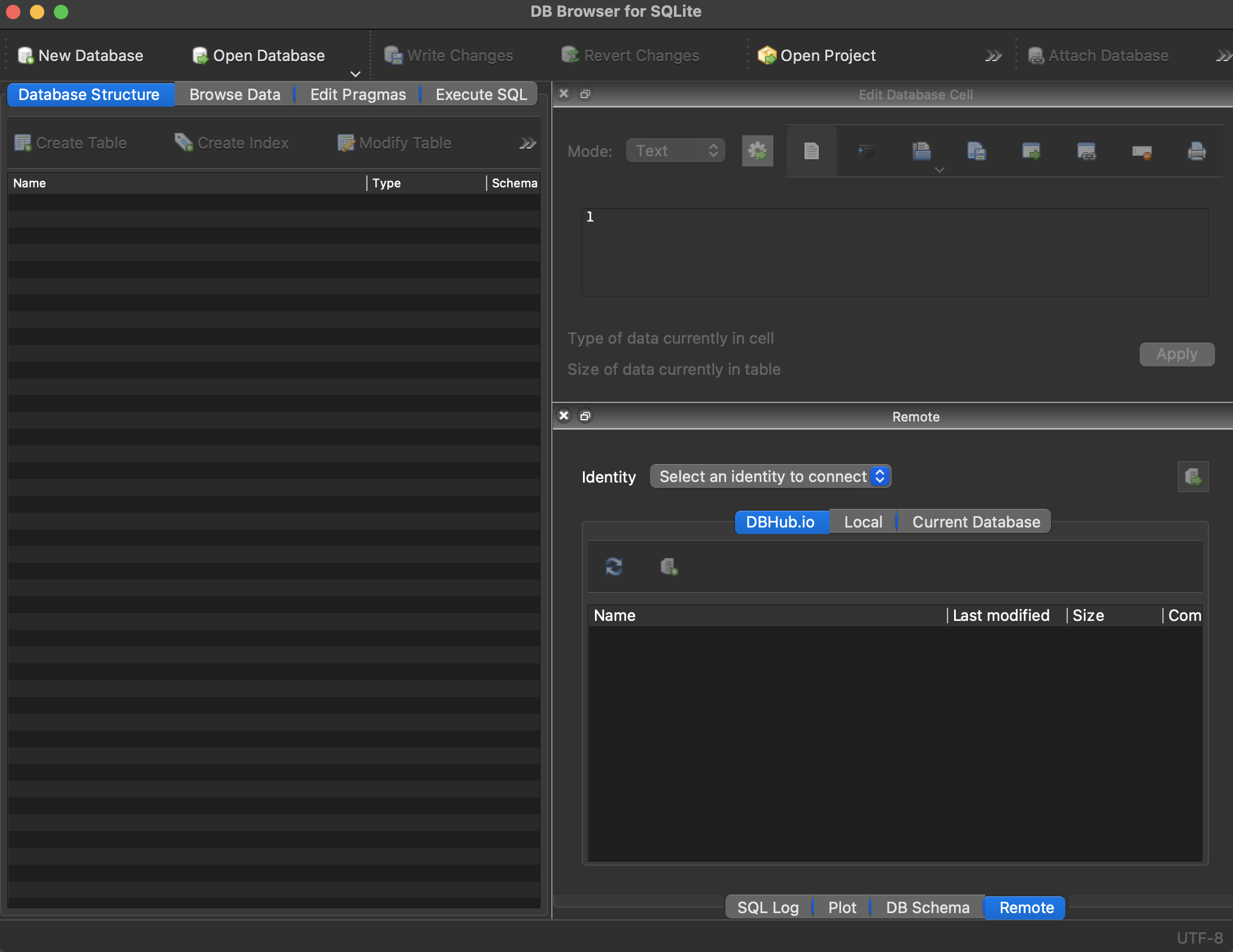
H.2 Getting started
To get started with SQL, download DB Browser for SQLite (DB4S), which is free and open source, and open it (Figure H.1).
Download “AustralianPoliticians.db” here and then open it with “Open Database” and navigate to where you downloaded the database.
There are three key SQL commands that we now cover: SELECT, FROM, and WHERE. SELECT allows us to specify particular columns of the data, and we can consider SELECT in a similar way to select(). In the same way that we need to specify a dataset with select() and did that using a pipe operator, we specify a dataset with FROM. For instance, we could open “Execute SQL”, and then type the following, and click “Execute”.
The result is that we obtain the column of surnames. We could select multiple columns by separating them with commas, or all of them by using an asterisk, although this is not best practice because if the dataset were to change without us knowing then our result would differ.
SELECT
    uniqueID,
    surname
FROM
    politicians;
SELECT
*
FROM
politicians;And, finally, if there were repeated rows, then we could just look at the unique ones using DISTINCT, in a similar way to distinct().
SELECT
    DISTINCT surname
FROM
    politicians;
So far we have used SELECT along with FROM. The third command that is commonly used is WHERE, and this will allow us to focus on particular rows, in a similar way to filter().
SELECT
    uniqueID,
    surname,
    firstName
FROM
    politicians
WHERE
    firstName = "Myles";
All the usual logical operators are fine with WHERE, such as “=”, “!=”, “>”, “<”, “>=”, and “<=”. We could combine conditions using AND and OR.
SELECT
    uniqueID,
    surname,
    firstName
FROM
    politicians
WHERE
    firstName = "Myles"
    OR firstName = "Ruth";
If we have a query that gave a lot of results, then we could limit the number of them with LIMIT.
SELECT
    uniqueID,
    surname,
    firstName
FROM
    politicians
WHERE
    firstName = "Robert"       LIMIT 5;
And we could specify the order of the results with ORDER.
SELECT
    uniqueID,
    surname,
    firstName
FROM
    politicians
WHERE
    firstName = "Robert"
ORDER BY
    surname DESC;
See the rows that are pretty close to a criteria:
SELECT
    uniqueID,
    surname,
    firstName
FROM
    politicians
WHERE
    firstName LIKE "Ma__";
The “_” above is a wildcard that matches to any character. This provides results that include “Mary” and “Mark”. LIKE is not case-sensitive: “Ma__” and “ma__” both return the same results.
Focusing on missing data is possible using “NULL” or “NOT NULL”.
SELECT
    uniqueID,
    surname,
    firstName,
    comment
FROM
    politicians
WHERE
    comment     IS NULL;
An ordering is applied to number, date, and text fields that means we can use BETWEEN on all those, not just numeric. For instance, we could look for all surnames that start with a letter between X and Z (not including Z).
SELECT
    uniqueID,
    surname,
    firstName
FROM
    politicians
WHERE
    surname     BETWEEN "X" AND "Z";
Using WHERE with a numeric variable means that BETWEEN is inclusive, compared with the example with letters which is not.
SELECT
    uniqueID,
    surname,
    firstName,
    birthYear
FROM
    politicians
WHERE
    birthYear     BETWEEN 1980 AND 1990;
In addition to providing us with dataset observations that match what we asked for, we can modify the dataset. For instance, we could edit a value using UPDATE and SET.
UPDATE
    politicians
SET
    displayName = "John Gilbert Alexander"
WHERE
    uniqueID = "Alexander1951";
We can integrate if-else logic with CASE and ELSE. For instance, we add a column called “wasTreasurer”, which is “Yes” in the case of “Josh Frydenberg”, and “No” in the case of “Kevin Rudd”, and “Unsure” for all other cases.
SELECT
    uniqueID,
    surname,
    firstName,
    birthYear,
    CASE
        WHEN uniqueID = "Frydenberg1971" THEN "Yes"
        WHEN surname = "Rudd" THEN "No"
        ELSE "Unsure"
    END AS "wasTreasurer"
FROM
    politicians;
We can create summary statistics using commands such as COUNT, SUM, MAX, MIN, AVG, and ROUND in the place of summarize(). COUNT counts the number of rows that are not empty for some column by passing the column name, and this is similarly how MIN, etc, work.
SELECT
    COUNT(uniqueID)
FROM
    politicians;
SELECT
MIN(birthYear)
FROM
politicians;We can get results based on different groups in our dataset using GROUP BY, in a similar manner to group_by in R.
SELECT
    COUNT(uniqueID)
FROM
    politicians
GROUP BY
    gender;
And finally, we can combine two tables using LEFT JOIN. We need to be careful to specify the matching columns using dot notation.
SELECT
    politicians.uniqueID,
    politicians.firstName,
    politicians.surname,
    party.partySimplifiedName
FROM
    politicians
LEFT JOIN
    party
        ON politicians.uniqueID = party.uniqueID;
As SQL is not our focus we have only provided a brief overview of some essential commands. From a career perspective you should develop a comfort with SQL. It is so integrated into data science that it would be “difficult to get too far without it” (Robinson and Nolis 2020, 8) and that “almost any” data science interview will include questions about SQL (Robinson and Nolis 2020, 110).
H.3 Exercises
Questions
- Please submit a screenshot showing you got at least 70 per cent in the free w3school SQL Quiz available here. You may like to go through their tutorial here. But the SQL content in this chapter is sufficient to get 70 per cent. Please include the time and date in the screenshot i.e. take a screenshot of your whole screen, not just the browser.