Online Appendix D — R Markdown

Quarto is the successor to R Markdown, however it is relatively new and many people still use R Markdown. For the most part, the aspects covered in Chapter 3 apply for both Quarto and R Markdown. However, in this appendix we provide an equivalent for R Markdown, for the guidance provided for Quarto, where there are aspects that differ.

D.1 R chunks

We can include code for R and many other languages in code chunks within an R Markdown document. Then when we knit the document, the code will run and be included in the document.

To create an R chunk, we start with three backticks and then within curly braces we tell R Markdown that this is an R chunk. Anything inside this chunk will be considered R code and run as such. For instance, we could load the tidyverse and AER and make a graph of the number of times a survey respondent visited the doctor in the past two weeks.

```{r}
library(tidyverse)
library(AER)

data("DoctorVisits", package = "AER")

DoctorVisits |>
  ggplot(aes(x = illness)) +
  geom_histogram(stat = "count")
```

The output of that code is Figure 3.1

Number of illnesses in the past two weeks, based on the 1977–1978 Australian Health Survey

Notice that in contrast to Quarto, all the options go between curly braces in the top line. It is not possible to use the comment notation of Quarto.

D.2 Cross-references

It can be useful to cross-reference figures, tables, and equations. This makes it easier to refer to them in the text. To do this for a figure we refer to the name of the R chunk that creates or contains the figure. For instance, (Figure \@ref(fig:uniquename)) will produce: (Figure 3.2) as the name of the R chunk is uniquename. We also need to add ‘fig’ in front of the chunk name so that R Markdown knows that this is a figure. We then include a ‘fig.cap’ in the R chunk that specifies a caption.

```{r uniquename, fig.cap = "Number of illnesses in the past two weeks, based on the 1977--1978 Australian Health Survey", echo = TRUE}

library(tidyverse)
library(AER)

data("DoctorVisits", package = "AER")

DoctorVisits |>
  ggplot(aes(x = illness)) +
  geom_histogram(stat = "count")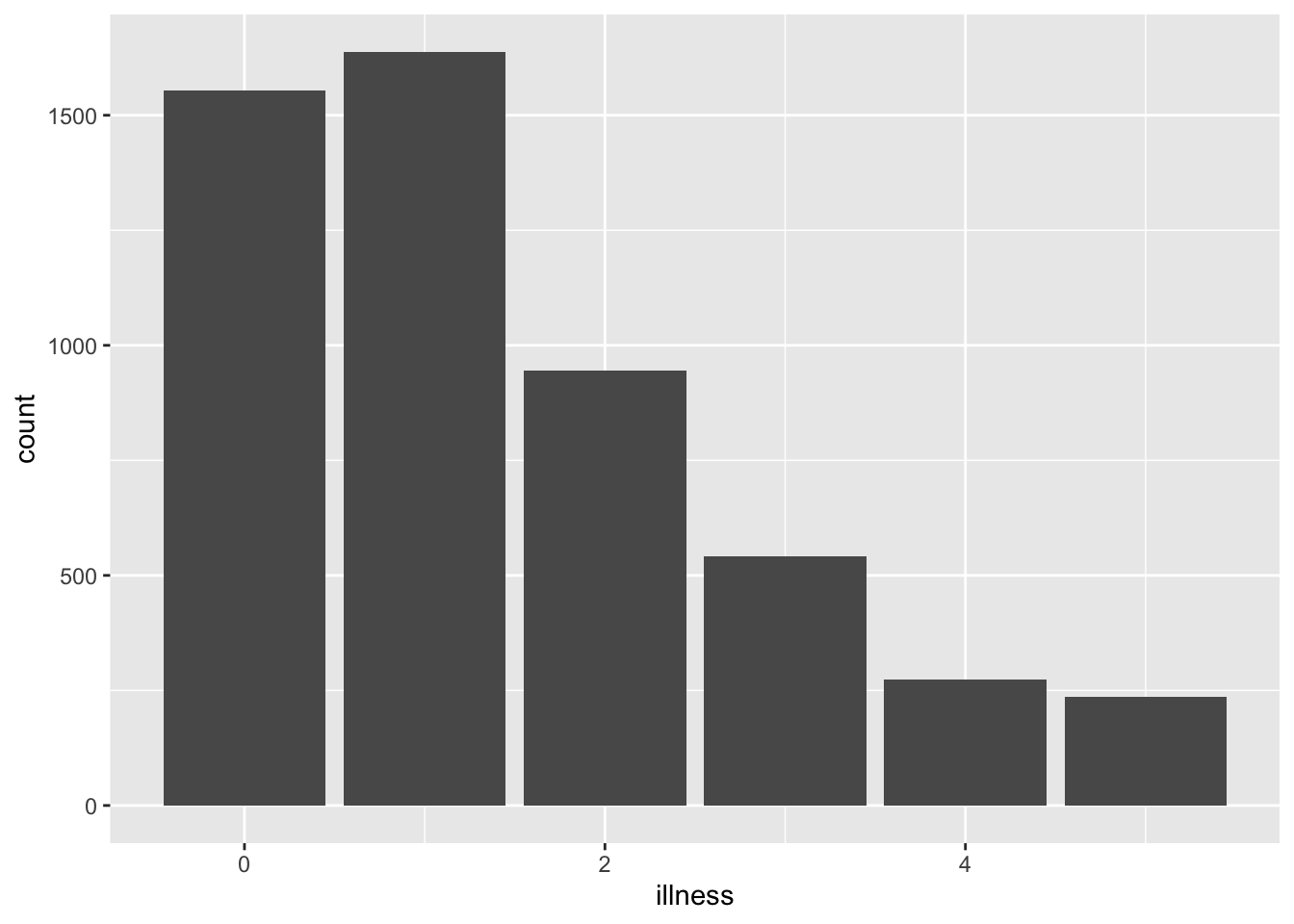

Number of illnesses in the past two weeks, based on the 1977–1978 Australian Health Survey

We can take a similar, but slightly different, approach to cross-reference tables. For instance, (Table \@ref(tab:docvisittablermarkdown)) will produce: (Table D.1). In this case we specify ‘tab’ before the unique reference to the table, so that R Markdown knows that it is a table. For tables we need to include the caption in the main content, as a ‘caption’, rather than in a ‘fig.cap’ chunk option as is the case for figures.

Table D.1: Number of visits to the doctor in the past two weeks, based on the 1977–1978 Australian Health Survey

visits	n
0	4141
1	782
2	174
3	30
4	24
5	9
6	12
7	12
8	5
9	1

Finally, we can also cross-reference equations. To that we need to add a tag (\#eq:macroidentity) which we then reference. For instance, use Equation \@ref(eq:macroidentity). to produce (Equation D.1)

\begin{equation}
Y = C + I + G + (X - M) (\#eq:macroidentity)
\end{equation}

\[ Y = C + I + G + (X - M) \tag{D.1}\]

When using cross-references ensure that the R chunks have simple labels. In general, try to keep the names simple but unique, and if possible, avoid punctuation and stick to letters. Do not use underbars in the labels because that will cause an error.